Classify Land Cover Using Hyperspectral and Lidar Data
This example shows how to classify land cover using a fusion of hyperspectral and lidar data.
This example requires the Hyperspectral Imaging Library for Image Processing Toolbox™. You can install the Hyperspectral Imaging Library for Image Processing Toolbox from Add-On Explorer. For more information about installing add-ons, see Get and Manage Add-Ons. The Hyperspectral Imaging Library for Image Processing Toolbox requires desktop MATLAB®, as MATLAB® Online™ and MATLAB® Mobile™ do not support the library.
This example uses data from the MUUFL Gulfport Data Set [1][2]. The MUUFL Gulfport Data Set comprises data acquired simultaneously by airborne hyperspectral and lidar sensors on an aircraft over the University of Southern Mississippi – Gulfport in November 2010. Because the hyperspectral and lidar data were acquired simultaneously, they are already spatially registered. The hyperspectral data provides information about the spectral properties of the land cover, whereas the lidar data provides information about the elevation of the land cover from the ground along with intensity information. You can fuse information from the hyperspectral and lidar data to classify land cover accurately.
In this example you perform these steps.
Load, visualize, and preprocess hyperspectral and lidar data.
Extract spatial features from the lidar data.
Fuse the hyperspectral and lidar data into a multichannel image.
Spatially split the fused multichannel image into training and test images.
Train a support vector machine (SVM) classifier on the training image.
Predict the class of land cover in the test image, and evaluate the classification accuracy.
Download Data Set
Download and unzip the data set.
zipFile = matlab.internal.examples.downloadSupportFile("image","data/gulfport_dataset.zip");
[filepath,folder,~] = fileparts(zipFile);
unzip(zipFile,filepath)
Load and Visualize Hyperspectral and Lidar Data
Load the hyperspectral data into the workspace as a hypercube object. The wavelength range of the hyperspectral data is 375 to 1050 nm [1][2]. Visualize an RGB image of the hyperspectral data.
filename = fullfile(filepath,folder,"gulfport_dataset","hyperspectralData.dat");
hcube = imhypercube(filename);
datacube = gather(hcube);
[rows,cols,bands] = size(datacube);
rgbImg = colorize(hcube,Method="rgb",ContrastStretching=true);
figure
imagesc(rgbImg)
title("RGB Image of Hyperspectral Data")
axis equal tight

Load the lidar data into the workspace as a lasFileReader (Lidar Toolbox) object. Read the point cloud from the lidar data, and visualize the locations and intensities of the points in the point cloud. The wavelength used to capture the lidar intensity is 1064 nm, which is outside the range of the wavelengths present in the hyperspectral data [1][2]. Observe that the intensity of the point cloud has some outliers.
filename = fullfile(filepath,folder,"gulfport_dataset","lidarData.las");
lasReader = lasFileReader(filename);
ptCloud = readPointCloud(lasReader);
ptCloudIntensity = reshape(ptCloud.Intensity,rows,cols);
figure
pcshow(ptCloud.Location)
title("Point Cloud of Lidar Data")
xlabel("X")
ylabel("Y")
zlabel("Z")

figure
imagesc(ptCloudIntensity)
title("Lidar Intensity")
axis equal tight
colorbar

Preprocess Hyperspectral and Lidar Data
Extract the hyperspectral data cube from the hyperspectral data and rescale it.
hyperspectralData = gather(hcube);
normHyperspectralData = rescale(hyperspectralData);
The lidar point cloud is unorganized, which means the data consists of rows of 3-D coordinates, each row representing a single point. To fuse the hyperspectral data to the lidar data, however, you must convert the lidar data to an organized point cloud. An organized point cloud separates the x-, y-, and z-coordinates of each point onto separate pages of a 3-D array, and divides the points based on their spatial relationships to one another. For more information on organized and unorganized point clouds, see What Are Organized and Unorganized Point Clouds? (Lidar Toolbox).
Organizing the locations of a point cloud requires information about the spatial relationships between the points. Since the hyperspectral and lidar data have already been registered, the locations of the points in the point cloud refer to the spatial locations of pixels in the hyperspectral image. Manually organize the point cloud using the spatial information of the points.
lidarElevation = ptCloud.Location(:,3);
lidarElevation = reshape(lidarElevation,rows,cols);
The three slices of the 3-D array lidarData refer to the x-, y-, and z-coordinates of the points in the point cloud. While the x- and y-coordinates refer to the spatial location of each point on the ground, the z-coordinate refers to the elevation of the point from the ground. Rescale the z-coordinate of the lidar data.
normLidarElevation = rescale(lidarElevation);
Remove the outliers from the intensity of the lidar data using a 2-D median filter. Observe that the outliers have been removed, and then rescale the lidar intensity data.
lidarIntensity = ptCloud.Intensity;
lidarIntensity = reshape(lidarIntensity,rows,cols);
lidarIntensity = medfilt2(lidarIntensity);
figure
imagesc(lidarIntensity)
title("Denoised Lidar Intensity")
axis equal tight
colorbar

normLidarIntensity = rescale(lidarIntensity);
Extract Spatial Features
Extract Gabor features from the rescaled lidar intensity data to incorporate spatial features in the classification.
gaborbank = gabor([2 4],[0 90]);
lidarGaborFeatures = imgaborfilt(normLidarIntensity,gaborbank);
Create Fused Hyperspectral Lidar Multichannel Image
The hyperspectral data and the intensity of the lidar data provide information about the spectral properties of the land cover, the features extracted using the Gabor filter bank provide spatial information, and the z-coordinate of the lidar data provides information about the elevation of the land cover from the ground.
You can fuse information from the hyperspectral and lidar data to classify land cover accurately by specifying selectData as "fused". By default, this example sets selectData to "fused", which fuses information from the hyperspectral and lidar data into a multichannel image. However, you can select one of these options to use only the hyperspectral data or only the lidar data.
"hyperspectral"— Use only the hyperspectral data."lidar"— Use only the lidar intensity data, lidar elevation data, and Gabor features extracted from lidar intensity.
selectData =
"fused"
selectData = "fused"
if isequal(selectData,"fused")
    data = cat(3,normHyperspectralData,normLidarIntensity,normLidarElevation,lidarGaborFeatures);
elseif isequal(selectData,"hyperspectral")
    data = normHyperspectralData;
elseif isequal(selectData,"lidar")
    data = cat(3,normLidarIntensity,normLidarElevation,lidarGaborFeatures);
end
Load Ground Truth Label Image
Load the ground truth labels into the workspace.
filename = fullfile(filepath,folder,"gulfport_dataset","labelData.mat");
load(filename,"labelData")
filename = fullfile(filepath,folder,"gulfport_dataset","labelDescriptions.mat");
load(filename,"labelDescriptions")
figure
imagesc(labelData)
axis equal tight
colorbar(Ticks=unique(labelData),TickLabels=labelDescriptions,TickLabelInterpreter="none")
title("Labels")
Create Training and Test Data Sets
Split the fused multichannel image into independent training and test images. Select the left 70% of the fused multichannel image as the training image and the right 30% of the fused multichannel image as the test image.
trainPercent = 0.7;
trainCol = floor(cols*trainPercent);
testCol = trainCol + 1;
trainImage = data(:,1:trainCol,:);
trainColsNum = size(trainImage,2);
testImage = data(:,testCol:end,:);
testColsNum = size(testImage,2);
Split the label image similarly to get a training label image and a test label image. Visualize the training and test label images separately.
trainLabels = labelData(:,1:trainCol);
testLabels = labelData(:,testCol:end);
figure
tiledlayout(1,2,InnerPosition=[0.1000 0.1100 0.7750 0.8150])
nexttile
imagesc(trainLabels)
axis equal tight
title("Training Labels")
nexttile
imagesc(testLabels)
axis equal tight
colorbar(Ticks=unique(labelData),TickLabels=labelDescriptions,TickLabelInterpreter="none")
title("Test Labels")

Prepare Data for Classification
To use the training and test images with a classifier model, reshape the images such that each row represents a pixel and each column represents a channel of the fused multichannel image.
trainData = reshape(trainImage,rows*trainColsNum,[]);
testData = reshape(testImage,rows*testColsNum,[]);
Reshape the training label image and test label image into single columns of data.
trainLabels = reshape(trainLabels,rows*trainColsNum,[]);
testLabels = reshape(testLabels,rows*testColsNum,[]);
Remove the unlabeled pixels from the training data.
unlabelTrain = trainLabels == -1;
trainData = trainData(~unlabelTrain,:);
trainLabels = trainLabels(~unlabelTrain);
Train SVM Classifier
Train a multiclass SVM classifier on the training data and labels by using the fitcecoc (Statistics and Machine Learning Toolbox) function.
rng("default")
model = fitcecoc(trainData,trainLabels,Learners="svm")
model =
  ClassificationECOC
             ResponseName: 'Y'
    CategoricalPredictors: []
               ClassNames: [1 2 3 4 5 6 7 8 9 10 11]
           ScoreTransform: 'none'
           BinaryLearners: {55×1 cell}
               CodingName: 'onevsone'


  Properties, Methods
Predict Labels of Test Data
Predict the labels of the test data using the trained multiclass SVM model.
predictedLabels = predict(model,testData);
Evaluate Classification Accuracy
Compute the accuracy of the predicted labels on the pixels for you have ground truth labels. The classification accuracy depends on the value of selectData.
If you set
selectDatato"fused", the classification accuracy is 80.67%.If you set
selectDatato"hyperspectral", the classification accuracy is 70.95%.If you set
selectDatato"lidar", the classification accuracy is 61.31%.
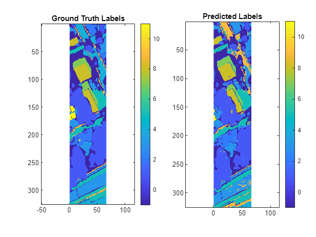
Observe that the classification accuracy improves significantly if you fuse the hyperspectral and lidar data, compared using the hyperspectral or lidar data individually.
unlabelTest = testLabels == -1;
predictedLabels(unlabelTest) = -1;
accuracy = nnz(predictedLabels(~unlabelTest)==testLabels(~unlabelTest)) / numel(testLabels(~unlabelTest))
accuracy =
0.8067
Reshape the test labels and the predicted labels into images, and visualize them.
testLabels = reshape(testLabels,rows,[]);
predictedLabels = reshape(predictedLabels,rows,[]);
figure
tiledlayout(1,2)
nexttile
imagesc(testLabels)
axis equal tight
title({"Ground Truth"; "Labels"})
nexttile
imagesc(predictedLabels)
axis equal tight
colorbar(Ticks=unique(labelData),TickLabels=labelDescriptions,TickLabelInterpreter="none")
title({"Predicted"; "Labels"})

References
[1] P. Gader, A. Zare, R. Close, J. Aitken, and G. Tuell. “MUUFL Gulfport Hyperspectral and LiDAR Airborne Data Set.” Technical Report REP-2013-570. University of Florida, Gainesville, 2013. https://github.com/GatorSense/MUUFLGulfport/tree/master.
[2] X. Du and A. Zare. “Technical Report: Scene Label Ground Truth Map for MUUFL Gulfport Data Set.” University of Florida, Gainesville, 2017. https://ufdc.ufl.edu/IR00009711/00001.
See Also
hypercube | lasFileReader (Lidar Toolbox) | fitcecoc (Statistics and Machine Learning Toolbox)