Classify Hyperspectral Image Using Support Vector Machine Classifier
This example shows how to perform hyperspectral image classification using a support vector machine (SVM) classifier.
This example requires the Hyperspectral Imaging Library for Image Processing Toolbox™. You can install the Hyperspectral Imaging Library for Image Processing Toolbox from Add-On Explorer. For more information about installing add-ons, see Get and Manage Add-Ons. The Hyperspectral Imaging Library for Image Processing Toolbox requires desktop MATLAB®, as MATLAB® Online™ and MATLAB® Mobile™ do not support the library.
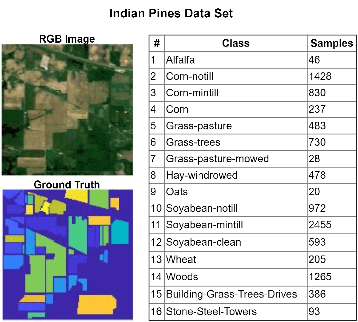
Hyperspectral images are acquired over multiple spectral bands and consist of several hundred band images, each representing the same scene across different wavelengths. This example uses the Indian Pines data set, acquired by the Airborne Visible/Infrared Imaging Spectrometer (AVIRIS) sensor across a wavelength range of 400 to 2500 nm. This data set contains 16 classes and 220 band images. Each image is of size 145-by-145 pixels.
In this example, you:
Preprocess a hyperspectral image using a 2-D Gaussian filter.
Perform classification using a SVM classifier.
Display classification results, such as the classification accuracy, classification map, and confusion matrix.
Load Hyperspectral Data Set
Read the hyperspectral data into the workspace.
hcube = imhypercube("indian_pines.dat");Load the ground truth for the data set into the workspace.
gtLabel = load("indian_pines_gt.mat");
gtLabel = gtLabel.indian_pines_gt;
numClasses = 16;
Preprocess Hyperspectral Data
Remove the water absorption bands from the data by using the removeBands function.
band = [104:108 150:163 220]; % Water absorption bands
newhcube = removeBands(hcube,BandNumber=band);
Estimate RGB images of the input hypercube by using the colorize function.
rgbImg = colorize(newhcube,method="rgb");Apply a Gaussian filter () to each band image of the hyperspectral data using the imgaussfilt function, and then convert them to grayscale images.
hsData = gather(newhcube);
[M,N,C] = size(hsData);
hsDataFiltered = zeros(size(hsData));
for band = 1:C
    bandImage = hsData(:,:,band);
    bandImageFiltered = imgaussfilt(bandImage,2);
    bandImageGray = mat2gray(bandImageFiltered);
    hsDataFiltered(:,:,band) = uint8(bandImageGray*255);
end
Prepare Data for Classification
Reshape the filtered hyperspectral data to a set of feature vectors containing filtered spectral responses for each pixel.
DataVector = reshape(hsDataFiltered,[M*N C]);
Reshape the ground truth image to a vector containing class labels.
gtVector = gtLabel(:);
Find the location indices of the ground truth vector that contain class labels. Discard labels with the value 0, as they are unlabeled and do not represent a class.
gtLocs = find(gtVector~=0);
classLabel = gtVector(gtLocs);
Create training and testing location indices for the specified training percentage by using the cvpartition (Statistics and Machine Learning Toolbox) function.
per = 0.1; % Training percentage
cv = cvpartition(classLabel,HoldOut=1-per);
Split the ground truth location indices into training and testing location indices.
locTrain = gtLocs(cv.training);
locTest = gtLocs(~cv.training);
Classify Using SVM
Train the SVM classifier using the fitcecoc (Statistics and Machine Learning Toolbox) function.
svmMdl = fitcecoc(DataVector(locTrain,:),gtVector(locTrain,:));
Test the SVM classifier using the test data.
[svmLabelOut,~] = predict(svmMdl,DataVector(locTest,:));
Display Classification Results
Calculate and display the classification accuracy.
svmAccuracy = sum(svmLabelOut == gtVector(locTest))/numel(locTest);
disp(["Overall Classification Accuracy (%) = ",num2str(svmAccuracy.*100)])
"Overall Classification Accuracy (%) = " "95.9996"
Create an SVM classification map.
svmPredLabel = gtLabel;
svmPredLabel(locTest) = svmLabelOut;
Display the RGB image, ground truth map, and SVM classification map.
cmap = parula(numClasses);
figure
montage({rgbImg,gtLabel,svmPredLabel},cmap,Size=[1 3],BorderSize=10)
title("RGB Image | Ground Truth Map | SVM Classification Map")
% Specify the intensity limits for the colorbar
minR = min(min(gtLabel(:)),min(svmPredLabel(:)));
maxR = max(max(gtLabel(:)),max(svmPredLabel(:)));
clim([minR maxR])
colorbar
Display the confusion matrix.
fig = figure;
confusionchart(gtVector(locTest),svmLabelOut,ColumnSummary="column-normalized")
fig_Position = fig.Position;
fig_Position(3) = fig_Position(3)*1.5;
fig.Position = fig_Position;
title("Confusion Matrix: SVM Classification Results")

References
[1] Patro, Ram Narayan, Subhashree Subudhi, Pradyut Kumar Biswal, and Fabio Dell’acqua. “A Review of Unsupervised Band Selection Techniques: Land Cover Classification for Hyperspectral Earth Observation Data.” IEEE Geoscience and Remote Sensing Magazine 9, no. 3 (September 2021): 72–111. https://doi.org/10.1109/MGRS.2021.3051979.
See Also
hypercube | colorize | removeBands | fitcecoc (Statistics and Machine Learning Toolbox) | confusionchart (Statistics and Machine Learning Toolbox) | imgaussfilt