Reduced Order Modeling of a Nonlinear Dynamical System as an Identified Linear Parameter Varying Model
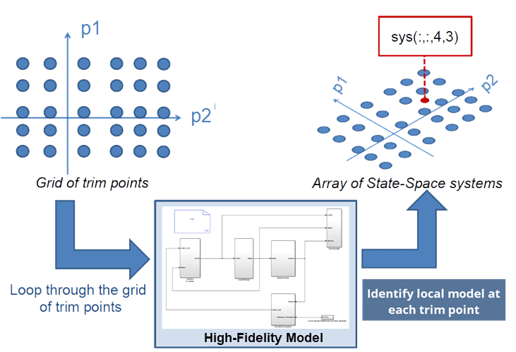
This example shows reduced order modeling (ROM) of a nonlinear system using a linear parameter varying (LPV) modeling technique. The nonlinear system used to describe the approach is a cascade of nonlinear mass-spring-damper systems. The development of the reduced order model is based on the idea of obtaining an array of linear models over the operating range of the nonlinear model by means of linearization or linear model identification. These local linear models are stitched together using interpolation techniques to produce a linear parameter-varying representation. Such representations are useful for generating faster-simulating proxies as well as for control design.
For the purpose of local model computation, the operating space is characterized by a set of scheduling parameters (p1, p2 in the diagram below). These parameters are varied over a grid of pre-chosen values. An equilibrium operating condition corresponding to each grid point is first determined by a model trimming exercise (see findop in Simulink® Control Design™). At each operating point, local perturbation experiments are performed to obtain a linear approximation of the system dynamics. The local models thus obtained are used to create a grid-based LPV model. This example requires that all the local models have matching structures. In particular, they must all use same state definitions. This example uses a Proper Orthogonal Decomposition (POD) approach to project the measured local responses into a common lower-dimensional space. The projected state trajectories are used to create lower-order state-space models using Dynamic Mode Decomposition (DMD).
The example uses a nonlinear mass-spring-damper Simulink model as the reference high-fidelity system. This system exhibits nonlinear stiffness and damping forces; such forces are polynomial functions of the mass displacement. The development of the LPV model follows these steps:
The nonlinear model is trimmed over a range of displacement values.
At each trim point, local small-signal simulations are performed and the data recorded.
These datasets are then used to create an array of linear state-space models. One-degree-of-freedom linear parameter varying model is simulated along a specific trajectory of the force . Multi-degree-of-freedom reduced order model is then obtained. The
n4sidcommand, which estimates a linear state space model from input-output data, is used to identify linear models for the equilibrium points of the cascade of mass-spring-damper systems.
Mass-Spring-Damper Model
Consider the single mass-spring-damper system (MSD) shown in the figure below, where is the mass, is the damping coefficient, is the stiffness coefficient of the spring, is the displacement of the mass from the equilibrium position, and and are input forces acting on the mass. represents a measurable disturbance and is a controllable input.
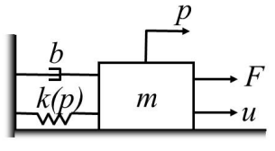
The MSD system can be modeled as in [1]:
where is the force due to spring stiffness and the damping force. Using the displacement and velocity as state variables, this equation can be put in the state-space form:
.
Defining and discretizing the above equation yields
.
Simplify the notation by using for leading to:
In this example, we consider the nonlinearity in the stiffness and the damping forces described by polynomials:
,
and the damping coefficient given by
,
where (stiffening spring). Let denote a time-varying operating condition that you use for scheduling the nonlinear dynamics. For this example, you schedule the behavior on different values of the disturbance force, that is, . If and the disturbance force is held constant at then the mass moves to an equilibrium position . This equilibrium position can be determined by solving the cubic equation for . Note that the damping force is zero at the equilibrium. Thus a parameterized collection of equilibrium conditions for the mass spring damper system is:
.
Linearizing this equation about the equilibrium conditions corresponding to a fixed value of yields:
where:
.
The linearized spring constant at the operating condition is . Similarly, (since zero velocity at equilibrium). For more details, see section 4.2 in [1].
The model considered for simulation in this example is a cascade of 100 masses connected with springs and dampers as shown in the figure above.
Local Analysis Using Perturbation Experiments
Set the values of the parameters required to simulate the MSD system. We consider , , , .
% System parameters
M = 100;        % Number of masses
m = 1;          % Mass of individual blocks, kg
k1 = 0.5;       % Linear spring constant, N/m
k2 = 1;         % Cubic spring constant, N/m^3
b1 = 1;         % Linear damping constant, N/(m/s)
b2 = 0.1;       % Cubic damping constant, N/(m/s)^3

% Model parameters
Tf = 20;        % simulation time
dt = 0.01;      % simulation time step (fixed step)
Experimental Setup
A perturbation experiment is performed on the MSD system with 100 masses as described in [1]. First, a collection of operating points are defined for the MSD system. Then, data is collected by running the simulation for each operating point.
% Initial condition
% (needed to update the size of x in mdl_NL)
x0 = zeros(M*2,1);

% Simulation times
dt = 0.1;           % Time step, sec
Tf = 20;
tin = 0:0.1:Tf;     % Time vector for snapshots, sec

% Select Parameter Grid
F_vec = (0:0.2:2)';
dut = [0 0];
dFt = [0 0];
F = F_vec(1);
U0 = 0;

Ngrid = numel(F_vec);
Nt = numel(tin);

% Batch trimming
params(1).Name = 'F';
params(1).Value = F_vec;
Create operating point specifications for the Simulink MSD_NL.slx model.
opspec = operspec('MSD_NL');
opopt = findopOptions('DisplayReport','off');
op = findop('MSD_NL',opspec, params, opopt);
Collect data at each grid point.
% Collect data at each grid point
xtrim = zeros(2*M,Ngrid);
dXall = zeros(2*M,Nt,Ngrid);
dUall = zeros(1,Nt,Ngrid);
dYall = zeros(1,Nt,Ngrid);
xOff = zeros(2*M,1,Ngrid);
yOff = zeros(1,1,Ngrid);

for i=1:Ngrid
   % Grab current grid point
   F = F_vec(i);
   U0 = 0;
   xtrim(:,i) = op(i).States.x;

   % Excite nonlinear system with chirp input, u
   w0 = 0.1;
   wf = 1+F;
   win = w0*(wf/w0).^(tin/Tf);
   uin = 1e-1*sin( win.*tin );

   dut = [tin(:) uin(:)];
   dFt = [0, 0; Tf, 0];

   % Simulate using Simulink model
   x0 = op(i).States.x;
   simout_NL_perturb = sim('MSD_NL');
   states = simout_NL_perturb.simout.Data;
   states = (squeeze(states))';

   % Collect snapshots
   dXall(:,:,i) = states'-repmat(x0,[1 Nt]);
   dUall(:,:,i) = uin;
   % note that the 100th state is treated as model output
   dYall(:,:,i) = dXall(M,:,i);

   % Collect offset data (input offset is 0)
   xOff(:,:,i) = op(i).States.x;
   yOff(:,:,i) = op(i).States.x(M);
end
Reduced-Order Linear Parameter Varying Modeling
Perform reduced-order modeling using linear parameter varying models, where the local models are obtained using Dynamic Mode Decomposition (DMD).
X = dXall;
Y = dYall;
U = dUall;

Nx = size(X,1);
Nu = size(U,1);
Ny = size(Y,1);
Ngrid = size(X,3);
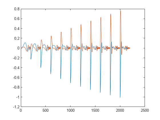
Concatenate the state trajectories from individual grid points along time, for PCA-type projection of the states.
% Concatenate the Ngrid (=1) state trajectories
% along the time (second) dimension.
X0all = reshape(X(:,1:end-1,:),Nx,[]);

% Plot a few for verification
plot(X0all([100 200],:)')
% POD modes using all state snapshots
[UU,SS,~] = svd(X0all);
Analyze the singular values in SS to determine a suitable projection dimension.
bar(diag(SS))
xlim([0 10])
ylabel('Singular values')
xlabel('Order')
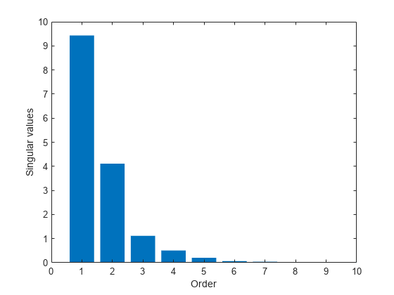
The plot suggests, roughly, a fifth order model. Project the state trajectories obtained over the grid into a 5-dimensional space.
% Select modes for subspace projection
Q = UU(:,1:5);

% Project all the state trajectories into the 5-dimensional space
Xs = pagemtimes(Q',X);
The projected state data Xs and the corresponding input and output trajectories at each grid point can be used in an identification algorithm to create the local linear models. In this example, we pose the identification problem as one of performing one-step prediction of the state and output trajectories:
Here, and are measured quantities. Hence the values of the unknowns can be obtained by linear regression. This scheme is a form of dynamic mode decomposition (DMD) that is often employed for the study of fluid dynamics - the DMD modes and eigenvalues describe the dynamics observed in the time series in terms of oscillatory components. The DMD technique is used to obtain separate linear models at each grid point.
% Generate values for Xs(t+1), and Xs(t) over a time span
% Time is along the second dimension in the variables Xs, Y, U
Xs_future = Xs(:,2:end,:);    % Xs(t+1)
Xs_current = Xs(:,1:end-1,:); % Xs(t)
Y_current = Y(:,1:end-1,:);   % Y(t)
U_current = U(:,1:end-1,:);   % U(t)

H = cat(1,Xs_future,Y_current);  % response to be predicted
R = cat(1,Xs_current,U_current); % regressor data ("predictor")

% Compute parameter estimates by linear regression
ABCD = pagemrdivide(H,R);
A = ABCD(1:5,1:5,:);
B = ABCD(1:5,6:end,:);
C = ABCD(6:end,1:5,:);
D = ABCD(6:end,6:end,:);

% Create a state space model array
% to represent the dynamics over the entire grid
Gred = ss(A,B,C,D,dt)
Gred(:,:,1,1) =

  A =
               x1          x2          x3          x4          x5
   x1      0.9968        -0.1     0.01319    0.009131   -0.004158
   x2      0.0598      0.8173      0.2205      0.1001     -0.3144
   x3    0.003302      0.0785      0.7367     0.04445      0.2369
   x4    -0.00134     0.01687    -0.09067      0.9168     0.09428
   x5  -0.0004078   -0.003254     0.04517     0.08203      0.8705

  B =
               u1
   x1  -1.956e-05
   x2      0.1129
   x3    -0.03799
   x4   -0.009784
   x5    0.004311

  C =
            x1       x2       x3       x4       x5
   y1  -0.9049  0.08258  0.03128   0.3008   0.2373

  D =
               u1
   y1  -0.0006643


Gred(:,:,2,1) =

  A =
              x1         x2         x3         x4         x5
   x1     0.9969    -0.1001    0.01301   0.008776  -0.004979
   x2    0.07983     0.8193     0.2194    0.04261    -0.4338
   x3  -0.004858    0.07868     0.7395    0.07153     0.2777
   x4  -0.002761    0.01683   -0.08896     0.9178    0.09539
   x5  0.0007509  -0.003889    0.04217    0.08096     0.8763

  B =
               u1
   x1  -5.993e-05
   x2      0.1087
   x3    -0.03629
   x4   -0.009364
   x5    0.003973

  C =
            x1       x2       x3       x4       x5
   y1  -0.9046  0.08234  0.03654   0.2987   0.2158

  D =
               u1
   y1  -0.0003161


Gred(:,:,3,1) =

  A =
              x1         x2         x3         x4         x5
   x1     0.9972    -0.1003    0.01283   0.008032   -0.00663
   x2      0.121     0.8147     0.2297  -0.009268    -0.6053
   x3   -0.02094    0.08264     0.7379    0.09681     0.3403
   x4  -0.005489    0.01761   -0.08895     0.9193     0.1044
   x5   0.002551  -0.005922    0.04063    0.07858     0.8736

  B =
               u1
   x1  -6.534e-05
   x2      0.1081
   x3    -0.03621
   x4   -0.009317
   x5    0.004041

  C =
            x1       x2       x3       x4       x5
   y1  -0.9035  0.08259  0.03938   0.2953   0.2003

  D =
               u1
   y1  -0.0001989


Gred(:,:,4,1) =

  A =
              x1         x2         x3         x4         x5
   x1     0.9974    -0.1006    0.01263   0.006901  -0.008381
   x2     0.1685     0.8085     0.2354   -0.05807    -0.7645
   x3   -0.03888    0.08726     0.7382     0.1219     0.3977
   x4  -0.008794    0.01842   -0.08986      0.924     0.1168
   x5   0.004541   -0.00794    0.04038    0.07137     0.8663

  B =
               u1
   x1  -7.154e-05
   x2      0.1082
   x3    -0.03629
   x4   -0.009334
   x5     0.00413

  C =
            x1       x2       x3       x4       x5
   y1  -0.9023  0.08265  0.04014   0.2957   0.1912

  D =
               u1
   y1  -0.0001015


Gred(:,:,5,1) =

  A =
              x1         x2         x3         x4         x5
   x1     0.9975    -0.1008    0.01234    0.00552  -0.009672
   x2     0.2145     0.8042     0.2269    -0.1153    -0.8794
   x3   -0.05591    0.09101     0.7432     0.1501      0.438
   x4   -0.01218     0.0189   -0.09013     0.9308     0.1265
   x5   0.006532  -0.009566     0.0403    0.06192     0.8605

  B =
               u1
   x1  -9.825e-05
   x2      0.1067
   x3     -0.0358
   x4   -0.009218
   x5    0.004116

  C =
            x1       x2       x3       x4       x5
   y1  -0.9014  0.08257   0.0395   0.2971   0.1851

  D =
               u1
   y1  -5.823e-05


Gred(:,:,6,1) =

  A =
             x1        x2        x3        x4        x5
   x1    0.9977   -0.1009   0.01201  0.004158  -0.01051
   x2    0.2563    0.8014    0.2105   -0.1711   -0.9568
   x3  -0.07114   0.09401    0.7507    0.1777    0.4641
   x4  -0.01535   0.01915  -0.08987    0.9375    0.1328
   x5  0.008356  -0.01088   0.04022   0.05266    0.8574

  B =
              u1
   x1  -0.000138
   x2     0.1041
   x3   -0.03488
   x4  -0.008992
   x5   0.004029

  C =
            x1       x2       x3       x4       x5
   y1  -0.9006   0.0824  0.03833   0.2983   0.1799

  D =
               u1
   y1  -3.959e-05


Gred(:,:,7,1) =

  A =
             x1        x2        x3        x4        x5
   x1    0.9978   -0.1011   0.01177  0.002849  -0.01165
   x2    0.2972    0.7973    0.1986   -0.2263     -1.06
   x3  -0.08582   0.09732    0.7562    0.2044    0.4979
   x4  -0.01854   0.01948  -0.09004    0.9438     0.141
   x5   0.01012   -0.0121   0.04049   0.04419    0.8545

  B =
               u1
   x1  -0.0001682
   x2      0.1021
   x3    -0.03416
   x4   -0.008821
   x5     0.00396

  C =
            x1       x2       x3       x4       x5
   y1     -0.9  0.08218    0.037   0.2987   0.1747

  D =
              u1
   y1  -3.35e-05


Gred(:,:,8,1) =

  A =
             x1        x2        x3        x4        x5
   x1    0.9979   -0.1013   0.01159  0.001579  -0.01285
   x2    0.3381    0.7918     0.189    -0.283    -1.173
   x3   -0.1003     0.101    0.7606    0.2311    0.5342
   x4  -0.02178   0.01991  -0.09041    0.9497    0.1496
   x5   0.01183  -0.01327   0.04099   0.03656    0.8523

  B =
               u1
   x1  -0.0001875
   x2      0.1008
   x3    -0.03371
   x4   -0.008723
   x5    0.003927

  C =
            x1       x2       x3       x4       x5
   y1  -0.8994  0.08194  0.03562   0.2985   0.1691

  D =
              u1
   y1  -3.29e-05


Gred(:,:,9,1) =

  A =
              x1         x2         x3         x4         x5
   x1     0.9979    -0.1015    0.01134  0.0004775   -0.01326
   x2     0.3734     0.7878     0.1718    -0.3315     -1.229
   x3    -0.1126     0.1039     0.7674     0.2543     0.5499
   x4   -0.02453    0.02018   -0.09004     0.9545     0.1525
   x5    0.01323   -0.01427    0.04122    0.03023     0.8538

  B =
               u1
   x1  -0.0002154
   x2     0.09881
   x3    -0.03301
   x4   -0.008556
   x5    0.003861

  C =
            x1       x2       x3       x4       x5
   y1  -0.8989  0.08168  0.03425   0.2976   0.1633

  D =
               u1
   y1  -3.545e-05


Gred(:,:,10,1) =

  A =
               x1          x2          x3          x4          x5
   x1      0.9978     -0.1016     0.01102  -0.0004348    -0.01298
   x2      0.4018      0.7859      0.1488     -0.3704      -1.237
   x3     -0.1225      0.1061       0.776      0.2735      0.5484
   x4    -0.02665     0.02024    -0.08908      0.9579      0.1503
   x5     0.01423     -0.0151     0.04123     0.02525      0.8588

  B =
               u1
   x1  -0.0002555
   x2     0.09582
   x3    -0.03197
   x4   -0.008294
   x5    0.003747

  C =
            x1       x2       x3       x4       x5
   y1  -0.8983  0.08141  0.03287   0.2963   0.1572

  D =
               u1
   y1  -4.082e-05


Gred(:,:,11,1) =

  A =
              x1         x2         x3         x4         x5
   x1     0.9978    -0.1017    0.01076  -0.001259   -0.01285
   x2     0.4298      0.783     0.1292    -0.4076     -1.264
   x3     -0.132     0.1085     0.7832     0.2914     0.5523
   x4   -0.02871    0.02038   -0.08841     0.9608     0.1493
   x5    0.01511    -0.0159    0.04148    0.02121     0.8642

  B =
               u1
   x1  -0.0002888
   x2     0.09334
   x3    -0.03111
   x4   -0.008077
   x5    0.003654

  C =
            x1       x2       x3       x4       x5
   y1  -0.8978  0.08113  0.03149   0.2945    0.151

  D =
               u1
   y1  -4.865e-05

Sample time: 0.1 seconds
11x1 array of discrete-time state-space models.
Model Properties
% Collect offset information
% (obtained earlier during operating point search)
Gred.SamplingGrid.F = F_vec; % scheduling parameter grid
Gred_offset_x = pagemtimes(Q',xOff);
Gred_offset_y = yOff;
bodemag(Gred) % frequency responses of the 11 models
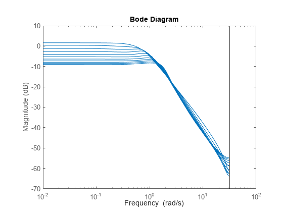
The LTI array Gred, along with the offset data can be used to create an LPV model. There are two ways of doing so:
In MATLAB® using the
ssInterpolantfunction to create anlvpssmodelIn Simulink using the LPV System block
LPV Model Creation and Simulation
Simulate the nonlinear and the linear parameter varying models with a sinusoidal input force and compare the results. First, simulate the original nonlinear system to generate the reference data.
Tf = 50;
tin = 0:dt:Tf;
Nt = numel(tin);

% Specify sinusoidal parameter (F) trajectory
amp = -1;
bias = 1;
freq = 0.5;
Ft = amp*cos(freq*tin)+bias;
dFt = [tin(:) Ft(:)];
F = 0;

% Specify input Force
dut = [tin(:) zeros(Nt,1)];
dut(tin>=25,2) = 0.1;
U0 = 0;

% Simulate the high-fidelity nonlinear model
simout_NL_MDOF = sim('MSD_NL');
tout = simout_NL_MDOF.tout;
simout_NL_MDOF_data = squeeze(simout_NL_MDOF.simout.Data)';
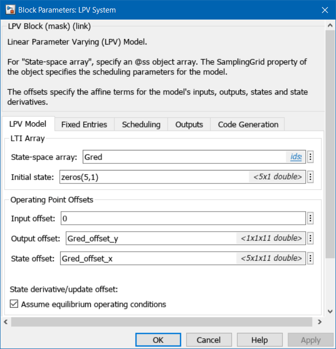
Simulate LPV Model in Simulink
Use the LPV System block to represent the LPV system. The block uses linear interpolation by default to interpolate the linear model matrices and the offsets.
% Simulate ROM LPV
open_system('MSD_MDOF_LPV')
simout_NL_MDOF_red = sim('MSD_MDOF_LPV');
simout_NL_MDOF_red_data = squeeze(simout_NL_MDOF_red.simout.Data);
ybar = simout_NL_MDOF_red_data(:,7);
Compare the responses of the original (MSD_NL) and the LPV approximation (MSD_MDOF_LPV).
% Compare the system output (position of the last mass)
plot(tout, simout_NL_MDOF_data(:,M),'b',...
   tout, simout_NL_MDOF_red_data(:,6),'r-.',...
   tout, ybar,'g:')
ylabel('Block 100 Position [m]');
xlabel('Time [sec]');
legend('Nonlinear model',...
   'LPV (Simulink)',...
   'Output offset (Trim)');
grid on;
![Figure contains an axes object. The axes object with xlabel Time [sec], ylabel Block 100 Position [m] contains 3 objects of type line. These objects represent Nonlinear model, LPV (Simulink), Output offset (Trim).](../../examples/ident/win64/ReducedOrderModelingOfANonlinearMSDSystemUsingIdentExample_07.png)
Simulate LPV Model in MATLAB
The LPV model is encapsulated by the lpvss object in MATLAB. The lpvss object supports simulations, and model operations such as c2d, feedback connection etc. When the LPV model is composed of an array of local linear models, the ssInterpolant command can be used to create the LPV model.
xc = squeeze(mat2cell(pagemtimes(Q',xOff),5,1,ones(1,Ngrid)));
yc = squeeze(mat2cell(yOff,1,1,ones(1,Ngrid)));
Offset = struct('dx',xc,'x',xc,'y',yc,'u',[]);
LPVModel = ssInterpolant(Gred, Offset)
Discrete-time state-space LPV model with 1 outputs, 1 inputs, 5 states, and 1 parameters.
Model Properties
Simulate LPVModel using the same input and scheduling trajectories as used for original nonlinear system. The simulation is performed using the lsim command.
Input = dut(:,2)+U0;
Time = dut(:,1);
Scheduling = dFt(:,2)+F;
x0 = zeros(5,1);
yLPV = lsim(LPVModel, Input, Time, x0, Scheduling);
plot(tout, simout_NL_MDOF_data(:,M),'b',...
   Time, yLPV,'r-.')
ylabel('Block 100 Position [m]');
xlabel('Time [sec]');
legend('Nonlinear model',...
   'LPV (MATLAB)');
grid on;
![Figure contains an axes object. The axes object with xlabel Time [sec], ylabel Block 100 Position [m] contains 2 objects of type line. These objects represent Nonlinear model, LPV (MATLAB).](../../examples/ident/win64/ReducedOrderModelingOfANonlinearMSDSystemUsingIdentExample_08.png)
The results show a good match between the original nonlinear system response, and that of its LPV approximation obtained by local linear modeling over a grid of scheduling values.
References
[1] Jennifer Annoni and Peter Seiler. "A method to construct reduced‐order parameter‐varying models." International Journal of Robust and Nonlinear Control 27.4 (2017): 582-597.