correct
Correct state and state estimation error covariance using extended or unscented Kalman filter, or particle filter and measurements
Syntax
Description
The correct command updates the state and state
estimation error covariance of an extendedKalmanFilter, unscentedKalmanFilter or particleFilter object using measured system outputs.
To implement extended or unscented Kalman filter, or particle filter, use the
correct and predict commands together. If the current output measurement exists, you
can use correct and predict. If the
measurement is missing, you can only use predict. For information
about the order in which to use the commands, see Using predict and correct Commands.
[ corrects the state
estimate and state estimation error covariance of an extended or unscented Kalman
filter, or particle filter object CorrectedState,CorrectedStateCovariance]
= correct(obj,y)obj using the measured output
y.
You create obj using the extendedKalmanFilter, unscentedKalmanFilter or particleFilter commands. You specify the state
transition function and measurement function of your nonlinear system in
obj. You also specify whether the process and measurement
noise terms are additive or nonadditive in these functions. The
State property of the object stores the latest estimated
state value. Assume that at time step k,
obj.State is . This value is the state estimate for time k,
estimated using measured outputs until time k-1. When you use the
correct command with measured system output
y[k], the software returns the corrected state estimate in the CorrectedState output. Where is the state estimate at time k, estimated
using measured outputs until time k. The command returns the
state estimation error covariance of in the CorrectedStateCovariance output. The
software also updates the State and
StateCovariance properties of obj with
these corrected values.
Use this syntax if the measurement function h that you
specified in obj.MeasurementFcn has one of the following forms:
y(k) = h(x(k))— for additive measurement noise.y(k) = h(x(k),v(k))— for nonadditive measurement noise.
Where y(k), x(k), and
v(k) are the measured output, states, and measurement noise
of the system at time step k. The only inputs to
h are the states and measurement noise.
[
specifies additional input arguments, if the measurement function of the system
requires these inputs. You can specify multiple arguments.CorrectedState,CorrectedStateCovariance]
= correct(obj,y,Um1,...,Umn)
Use this syntax if the measurement function h has one of the following forms:
y(k) = h(x(k),Um1,...,Umn)— for additive measurement noise.y(k) = h(x(k),v(k),Um1,...,Umn)— for nonadditive measurement noise.
correct command passes these inputs to the measurement
function to calculate the estimated outputs.
Examples
Estimate States Online Using Extended Kalman Filter
Estimate the states of a van der Pol oscillator using an extended Kalman filter algorithm and measured output data. The oscillator has two states and one output.
Create an extended Kalman filter object for the oscillator. Use previously written and saved state transition and measurement functions, vdpStateFcn.m and vdpMeasurementFcn.m. These functions describe a discrete-approximation to a van der Pol oscillator with the nonlinearity parameter equal to 1. The functions assume additive process and measurement noise in the system. Specify the initial state values for the two states as [1;0]. This is the guess for the state value at initial time k, based on knowledge of system outputs until time k-1, .
obj = extendedKalmanFilter(@vdpStateFcn,@vdpMeasurementFcn,[1;0]);
Load the measured output data y from the oscillator. In this example, use simulated static data for illustration. The data is stored in the vdp_data.mat file.
load vdp_data.mat y
Specify the process noise and measurement noise covariances of the oscillator.
obj.ProcessNoise = 0.01;
obj.MeasurementNoise = 0.16;
Initialize arrays to capture results of the estimation.
residBuf = [];
xcorBuf = [];
xpredBuf = [];
Implement the extended Kalman filter algorithm to estimate the states of the oscillator by using the correct and predict commands. You first correct using measurements at time k to get . Then, you predict the state value at the next time step using , the state estimate at time step k that is estimated using measurements until time k.
To simulate real-time data measurements, use the measured data one time step at a time. Compute the residual between the predicted and actual measurement to assess how well the filter is performing and converging. Computing the residual is an optional step. When you use residual, place the command immediately before the correct command. If the prediction matches the measurement, the residual is zero.
After you perform the real-time commands for the time step, buffer the results so that you can plot them after the run is complete.
for k = 1:length(y)
    [Residual,ResidualCovariance] = residual(obj,y(k));
    [CorrectedState,CorrectedStateCovariance] = correct(obj,y(k));
    [PredictedState,PredictedStateCovariance] = predict(obj);

     residBuf(k,:) = Residual;
     xcorBuf(k,:) = CorrectedState';
     xpredBuf(k,:) = PredictedState';

end
When you use the correct command, obj.State and obj.StateCovariance are updated with the corrected state and state estimation error covariance values for time step k, CorrectedState and CorrectedStateCovariance. When you use the predict command, obj.State and obj.StateCovariance are updated with the predicted values for time step k+1, PredictedState and PredictedStateCovariance. When you use the residual command, you do not modify any obj properties.
In this example, you used correct before predict because the initial state value was , a guess for the state value at initial time k based on system outputs until time k-1. If your initial state value is , the value at previous time k-1 based on measurements until k-1, then use the predict command first. For more information about the order of using predict and correct, see Using predict and correct Commands.
Plot the estimated states, using the post-correction values.
plot(xcorBuf(:,1), xcorBuf(:,2))
title('Estimated States')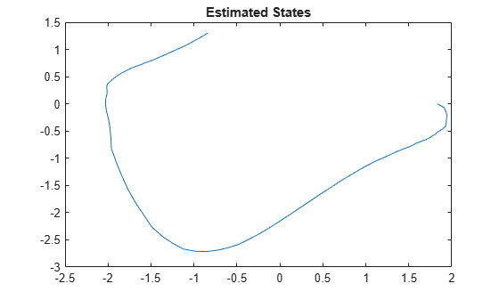
Plot the actual measurement, the corrected estimated measurement, and the residual. For the measurement function in vdpMeasurementFcn, the measurement is the first state.
M = [y,xcorBuf(:,1),residBuf];
plot(M)
grid on
title('Actual and Estimated Measurements, Residual')
legend('Measured','Estimated','Residual')
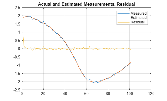
The estimate tracks the measurement closely. After the initial transient, the residual remains relatively small throughout the run.
Estimate States Online Using Particle Filter
Load the van der Pol ODE data, and specify the sample time.
vdpODEdata.mat contains a simulation of the van der Pol ODE with nonlinearity parameter mu=1, using ode45, with initial conditions [2;0]. The true state was extracted with sample time dt = 0.05.
load ('vdpODEdata.mat','xTrue','dt')
tSpan = 0:dt:5;
Get the measurements. For this example, a sensor measures the first state with a Gaussian noise with standard deviation 0.04.
sqrtR = 0.04;
yMeas = xTrue(:,1) + sqrtR*randn(numel(tSpan),1);
Create a particle filter, and set the state transition and measurement likelihood functions.
myPF = particleFilter(@vdpParticleFilterStateFcn,@vdpMeasurementLikelihoodFcn);
Initialize the particle filter at state [2; 0] with unit covariance, and use 1000 particles.
initialize(myPF,1000,[2;0],eye(2));
Pick the mean state estimation and systematic resampling methods.
myPF.StateEstimationMethod = 'mean';
myPF.ResamplingMethod = 'systematic';
Estimate the states using the correct and predict commands, and store the estimated states.
xEst = zeros(size(xTrue));
for k=1:size(xTrue,1)
    xEst(k,:) = correct(myPF,yMeas(k));
    predict(myPF);
end
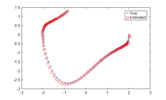
Plot the results, and compare the estimated and true states.
figure(1)
plot(xTrue(:,1),xTrue(:,2),'x',xEst(:,1),xEst(:,2),'ro')
legend('True','Estimated')
Specify State Transition and Measurement Functions with Additional Inputs
Consider a nonlinear system with input u whose state x and measurement y evolve according to the following state transition and measurement equations:
The process noise w of the system is additive while the measurement noise v is nonadditive.
Create the state transition function and measurement function for the system. Specify the functions with an additional input u.
f = @(x,u)(sqrt(x+u));
h = @(x,v,u)(x+2*u+v^2);
f and h are function handles to the anonymous functions that store the state transition and measurement functions, respectively. In the measurement function, because the measurement noise is nonadditive, v is also specified as an input. Note that v is specified as an input before the additional input u.
Create an extended Kalman filter object for estimating the state of the nonlinear system using the specified functions. Specify the initial value of the state as 1 and the measurement noise as nonadditive.
obj = extendedKalmanFilter(f,h,1,'HasAdditiveMeasurementNoise',false);Specify the measurement noise covariance.
obj.MeasurementNoise = 0.01;
You can now estimate the state of the system using the predict and correct commands. You pass the values of u to predict and correct, which in turn pass them to the state transition and measurement functions, respectively.
Correct the state estimate with measurement y[k]=0.8 and input u[k]=0.2 at time step k.
correct(obj,0.8,0.2)
Predict the state at the next time step, given u[k]=0.2.
predict(obj,0.2)
Retrieve the error, or residual, between the prediction and the measurement.
[Residual, ResidualCovariance] = residual(obj,0.8,0.2);
Input Arguments
Output Arguments
More About
Version History
Introduced in R2016b
See Also
predict | clone | extendedKalmanFilter | unscentedKalmanFilter | particleFilter | initialize | residual
You can also select a web site from the following list:
Americas
- América Latina (Español)
- Canada (English)
- United States (English)
Europe
- Belgium (English)
- Denmark (English)
- Deutschland (Deutsch)
- España (Español)
- Finland (English)
- France (Français)
- Ireland (English)
- Italia (Italiano)
- Luxembourg (English)
- Netherlands (English)
- Norway (English)
- Österreich (Deutsch)
- Portugal (English)
- Sweden (English)
- Switzerland
- United Kingdom (English)