Population Diversity
Importance of Population Diversity
One of the most important factors that determines the performance of the genetic algorithm performs is the diversity of the population. If the average distance between individuals is large, the diversity is high; if the average distance is small, the diversity is low. Getting the right amount of diversity is a matter of trial and error. If the diversity is too high or too low, the genetic algorithm might not perform well.
This section explains how to control diversity by setting the initial range of the population. The topic "Setting the Amount of Mutation" in Vary Mutation and Crossover describes how the amount of mutation affects diversity.
This section also explains how to set the population size.
Set Initial Range
By default, ga creates a random initial population using a creation function. You can specify the range of the vectors in the initial population in the InitialPopulationRange option.
Note: The initial range restricts the range of the points in the initial population by specifying the lower and upper bounds. Subsequent generations can contain points whose entries do not lie in the initial range. Set upper and lower bounds for all generations using the lb and ub input arguments.
If you know approximately where the solution to a problem lies, specify the initial range so that it contains your guess for the solution. However, the genetic algorithm can find the solution even if it does not lie in the initial range, if the population has enough diversity.
This example shows how the initial range affects the performance of the genetic algorithm. The example uses Rastrigin's function, described in Minimize Rastrigin's Function. The minimum value of the function is 0, which occurs at the origin.
rng(1) % For reproducibility
fun = @rastriginsfcn;
nvar = 2;
options = optimoptions("ga",PlotFcn={"gaplotbestf","gaplotdistance"},...
    InitialPopulationRange=[1;1.1]);
[x,fval] = ga(fun,nvar,[],[],[],[],[],[],[],options)
ga stopped because the average change in the fitness value is less than options.FunctionTolerance.
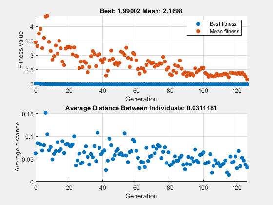
x = 1×2

    0.9942    0.9950
fval =
1.9900
The upper plot, which displays the best fitness at each generation, shows little progress in lowering the fitness value. The lower plot shows the average distance between individuals at each generation, which is a good measure of the diversity of a population. For this setting of initial range, there is too little diversity for the algorithm to make progress.
Next, try setting the InitialPopulationRange to [1;100]. This time the results are more variable. The current random number setting causes a fairly typical result.
options.InitialPopulationRange = [1;100];
[x,fval] = ga(fun,nvar,[],[],[],[],[],[],[],options)
ga stopped because the average change in the fitness value is less than options.FunctionTolerance.
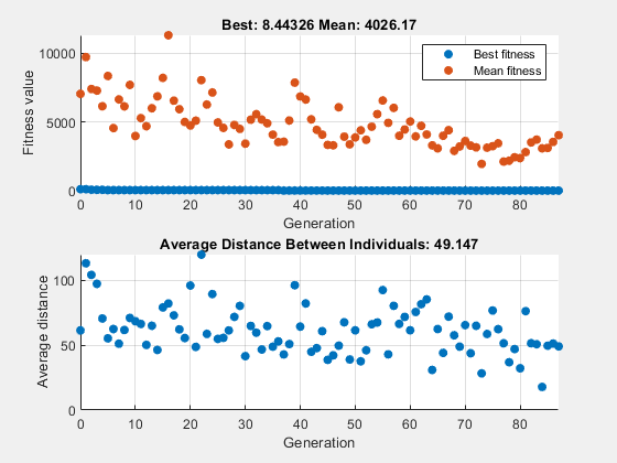
x = 1×2

   -2.1352   -0.0497
fval =
8.4433
This time, the genetic algorithm makes progress, but because the average distance between individuals is so large, the best individuals are far from the optimal solution.
Now set the InitialPopulationRange to [1;2]. This setting is well-suited to the problem.
options.InitialPopulationRange = [1;2];
[x,fval] = ga(fun,nvar,[],[],[],[],[],[],[],options)
ga stopped because it exceeded options.MaxGenerations.
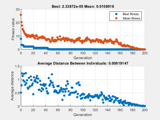
x = 1×2
10-3 ×

    0.2473   -0.2382
fval =
2.3387e-05
The suitable diversity usually causes ga to return a better result than in the previous two cases.
Custom Plot Function and Linear Constraints in ga
This example shows how @gacreationlinearfeasible, the default creation function for linearly constrained problems, creates a population for ga. The population is well-dispersed, and is biased to lie on the constraint boundaries. The example uses a custom plot function.
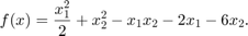
Fitness Function
The fitness function is lincontest6, which is available when you run this example. lincontest6 is a quadratic function of two variables:
Custom Plot Function
Save the following code to a file on your MATLAB® path named gaplotshowpopulation2.
function state = gaplotshowpopulation2(~,state,flag,fcn)
%gaplotshowpopulation2 Plots the population and linear constraints in 2-d.
%   STATE = gaplotshowpopulation2(OPTIONS,STATE,FLAG) plots the population
%   in two dimensions.
%
%   Example:
%     fun = @lincontest6;
%     options = gaoptimset(PlotFcn={{@gaplotshowpopulation2,fun}});
%     [x,fval,exitflag] = ga(fun,2,A,b,[],[],lb,[],[],options);

% This plot function works in 2-d only
if size(state.Population,2) > 2
    return;
end
if nargin < 4
    fcn = [];
end
% Dimensions to plot
dimensionsToPlot = [1 2];

switch flag
    % Plot initialization
    case "init"
        pop = state.Population(:,dimensionsToPlot);
        plotHandle = plot(pop(:,1),pop(:,2),"*");
        set(plotHandle,Tag="gaplotshowpopulation2")
        title("Population plot in two dimension",interp="none")
        xlabelStr = sprintf("%s %s",Variable = num2str(dimensionsToPlot(1)));
        ylabelStr = sprintf("%s %s",Variable = num2str(dimensionsToPlot(2)));
        xlabel(xlabelStr,interp="none");
        ylabel(ylabelStr,interp="none");
        hold on;

        % plot the inequalities
        plot([0 1.5],[2 0.5],"m-.") %  x1 + x2 <= 2
        plot([0 1.5],[1 3.5/2],"m-."); % -x1 + 2*x2 <= 2
        plot([0 1.5],[3 0],"m-."); % 2*x1 + x2 <= 3
        % plot lower bounds
        plot([0 0], [0 2],"m-."); % lb = [ 0 0];
        plot([0 1.5], [0 0],"m-."); % lb = [ 0 0];
        set(gca,xlim=[-0.7,2.2])
        set(gca,ylim=[-0.7,2.7])
        axx = gcf;
        % Contour plot the objective function
        if ~isempty(fcn)
            range = [-0.5,2;-0.5,2];
            pts = 100;
            span = diff(range')/(pts - 1);
            x = range(1,1): span(1) : range(1,2);
            y = range(2,1): span(2) : range(2,2);

            pop = zeros(pts * pts,2);
            values = zeros(pts,1);
            k = 1;
            for i = 1:pts
                for j = 1:pts
                    pop(k,:) = [x(i),y(j)];
                    values(k) = fcn(pop(k,:));
                    k = k + 1;
                end
            end
            values = reshape(values,pts,pts);
            contour(x,y,values);
            colorbar
        end
        % Show the initial population
        ax = gca;
        fig = figure;
        copyobj(ax,fig);colorbar
        % Pause for three seconds to view the initial plot, then resume
        figure(axx)
        pause(3);
    case "iter"
        pop = state.Population(:,dimensionsToPlot);
        plotHandle = findobj(get(gca,"Children"),Tag="gaplotshowpopulation2");
        set(plotHandle,Xdata=pop(:,1),Ydata=pop(:,2));
end
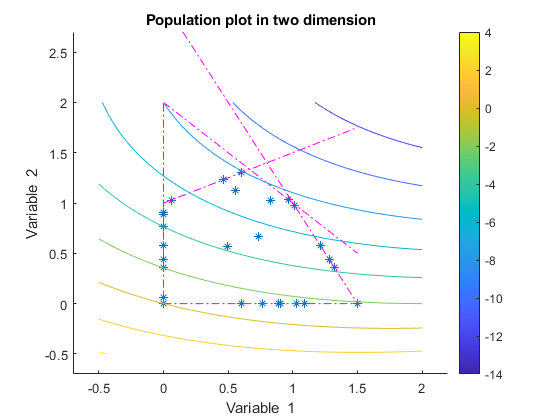
The custom plot function plots the lines representing the linear inequalities and bound constraints, plots level curves of the fitness function, and plots the population as it evolves. This plot function expects to have not only the usual inputs (options,state,flag), but also a function handle to the fitness function, @lincontest6 in this example. To generate level curves, the custom plot function needs the fitness function.
Problem Constraints
Include bounds and linear constraints.
A = [1,1;-1,2;2,1];
b = [2;2;3];
lb = zeros(2,1);
Options to Include Plot Function
Set options to include the plot function when ga runs.
options = optimoptions("ga",...
PlotFcn={{@gaplotshowpopulation2,@lincontest6}});
Run Problem and Observe Population
The initial population, in the first plot, has many members on the linear constraint boundaries. The population is reasonably well-dispersed.
rng default % for reproducibility
[x,fval] = ga(@lincontest6,2,A,b,[],[],lb,[],[],options);
ga stopped because the average change in the fitness value is less than options.FunctionTolerance.
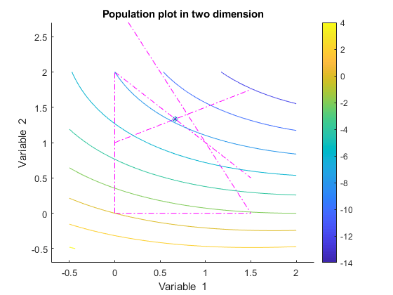
ga converges quickly to a single point, the solution.
Setting the Population Size
The Population size field in Population options determines the size of the population at each generation. Increasing the population size enables the genetic algorithm to search more points and thereby obtain a better result. However, the larger the population size, the longer the genetic algorithm takes to compute each generation.
Note
You should set Population size to be at least the value of Number of variables, so that the individuals in each population span the space being searched.
You can experiment with different settings for Population size that return good results without taking a prohibitive amount of time to run.