Implement Hardware-Efficient Real Burst Matrix Solve Using Q-less QR Decomposition with Tikhonov Regularization
This example shows how to use the Real Burst Matrix Solve Using QR Decomposition block to solve the regularized least-squares matrix equation
![$$\left[\begin{array}{c}\lambda I_n\\A\end{array}\right]^\mathrm{T} \left[\begin{array}{c}\lambda I_n\\A\end{array}\right]X = (\lambda^2I_n + A^\mathrm{T}A)X = B$$](../../examples/fixedpoint/win64/RealBurstRegularizedQlessQRMatrixSolveExample_eq09441744023426340016.png)
where A is an m-by-n matrix with m  n, B is n-by-p, X is n-by-p,
  , and
, and  is a regularization parameter.
Define System Parameters
Define the matrix attributes and system parameters for this example.
m is the number of rows in matrix A. In a problem such as beamforming or direction finding, m corresponds to the number of samples that are integrated over.
m = 100;
n is the number of columns in matrix A and rows in matrices B and X. In a least-squares problem, m is greater than n, and usually m is much larger than n. In a problem such as beamforming or direction finding, n corresponds to the number of sensors.
n = 10;
p is the number of columns in matrices B and X. It corresponds to simultaneously solving a system with p right-hand sides.
p = 1;
In this example, set the rank of matrix A to be less than the number of columns. In a problem such as beamforming or direction finding,  corresponds to the number of signals impinging on the sensor array.
rankA = 3;
precisionBits defines the number of bits of precision required for the matrix solve. Set this value according to system requirements.
precisionBits = 32;
Small, positive values of the regularization parameter can improve the conditioning of the problem and reduce the variance of the estimates. While biased, the reduced variance of the estimate often results in a smaller mean squared error when compared to least-squares estimates.
regularizationParameter = 0.01;
In this example, real-valued matrices A and B are constructed such that the magnitude of their elements is less than or equal to one. Your own system requirements will define what those values are. If you don't know what they are, and A and B are fixed-point inputs to the system, then you can use the upperbound function to determine the upper bounds of the fixed-point types of A and B.
max_abs_A is an upper bound on the maximum magnitude element of A.
max_abs_A = 1;
max_abs_B is an upper bound on the maximum magnitude element of B.
max_abs_B = 1;
Thermal noise standard deviation is the square root of thermal noise power, which is a system parameter. A well-designed system has the quantization level lower than the thermal noise. Here, set thermalNoiseStandardDeviation to the equivalent of -50 dB noise power.
thermalNoiseStandardDeviation = sqrt(10^(-50/10))
thermalNoiseStandardDeviation =

    0.0032
The quantization noise standard deviation is a function of the required number of bits of precision. Use fixed.realQuantizationNoiseStandardDeviation to compute this. See that it is less than thermalNoiseStandardDeviation.
quantizationNoiseStandardDeviation = fixed.realQuantizationNoiseStandardDeviation(precisionBits)
quantizationNoiseStandardDeviation =

   6.7212e-11
Compute Fixed-Point Types
In this example, assume that the designed system matrix  does not have full rank (there are fewer signals of interest than number of columns of matrix ), and the measured system matrix has additive thermal noise that is larger than the quantization noise. The additive noise makes the measured matrix have full rank.
Set  .
.
noiseStandardDeviation = thermalNoiseStandardDeviation;
Use the fixed.realQlessQRMatrixSolveFixedpointTypes function to compute fixed-point types.
T = fixed.realQlessQRMatrixSolveFixedpointTypes(m,n,max_abs_A,max_abs_B,...
    precisionBits,noiseStandardDeviation,[],regularizationParameter)
T =

  struct with fields:

    A: [0×0 embedded.fi]
    B: [0×0 embedded.fi]
    X: [0×0 embedded.fi]
T.A is the type computed for transforming ![$\left[\begin{array}{c}\lambda I_n\\A\end{array}\right]$](../../examples/fixedpoint/win64/RealBurstRegularizedQlessQRMatrixSolveExample_eq11993394244965770304.png) to
to ![$R=Q^\mathrm{T}\left[\begin{array}{c}\lambda I_n\\A\end{array}\right]$](../../examples/fixedpoint/win64/RealBurstRegularizedQlessQRMatrixSolveExample_eq17262898067175161434.png) in-place so that it does not overflow.
in-place so that it does not overflow.
T.A
ans =

[]

          DataTypeMode: Fixed-point: binary point scaling
            Signedness: Signed
            WordLength: 39
        FractionLength: 32
T.B is the type computed for B so that it does not overflow.
T.B
ans =

[]

          DataTypeMode: Fixed-point: binary point scaling
            Signedness: Signed
            WordLength: 35
        FractionLength: 32
T.X is the type computed for the solution ![$X = \left(\left[\begin{array}{c}\lambda I_n\\A\end{array}\right]^\mathrm{T} \left[\begin{array}{c}\lambda I_n\\A\end{array}\right]\right) \backslash B$](../../examples/fixedpoint/win64/RealBurstRegularizedQlessQRMatrixSolveExample_eq09998501448291651262.png) so that there is a low probability that it overflows.
so that there is a low probability that it overflows.
T.X
ans =

[]

          DataTypeMode: Fixed-point: binary point scaling
            Signedness: Signed
            WordLength: 50
        FractionLength: 32
Use the Specified Types to Solve the Matrix Equation
Create random matrices A and B such that rankA=rank(A). Add random measurement noise to A which will make it become full rank.
rng('default');
[A,B] = fixed.example.realRandomQlessQRMatrices(m,n,p,rankA);
A = A + fixed.example.realNormalRandomArray(0,noiseStandardDeviation,m,n);
Cast the inputs to the types determined by fixed.realQlessQRMatrixSolveFixedpointTypes. Quantizing to fixed-point is equivalent to adding random noise.
A = cast(A,'like',T.A);
B = cast(B,'like',T.B);
OutputType = fixed.extractNumericType(T.X);
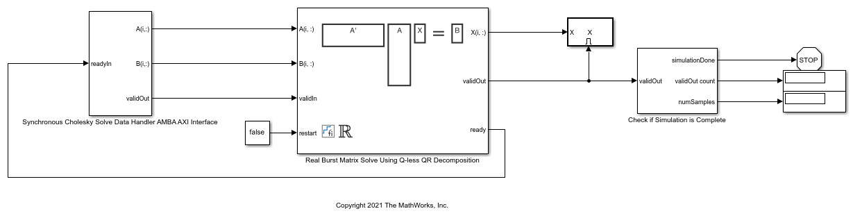
Open the Model
model = 'RealBurstQlessQRMatrixSolveModel';
open_system(model);
Set Variables in the Model Workspace
Use the helper function setModelWorkspace to add the variables defined above to the model workspace. These variables correspond to the block parameters for the Real Burst Matrix Solve Using QR Decomposition block.
numSamples = 1; % Number of sample matrices
rowDelay = 1; % Delay of clock cycles between feeding in rows of A and B
fixed.example.setModelWorkspace(model,'A',A,'B',B,'m',m,'n',n,'p',p,...
    'regularizationParameter',regularizationParameter,...
    'numSamples',numSamples,'rowDelay',rowDelay,'OutputType',OutputType);
Simulate the Model
out = sim(model);
Construct the Solution from the Output Data
The Real Burst Matrix Solve Using Q-less QR Decomposition block outputs data one row at a time. When a result row is output, the block sets validOut to true. The rows of X are output in the order they are computed, last row first, so you must reconstruct the data to interpret the results. To reconstruct the matrix X from the output data, use the helper function matrixSolveModelOutputToArray.
X = fixed.example.matrixSolveModelOutputToArray(out.X,n,p);
Verify the Accuracy of the Output
Verify that the relative error between the fixed-point output and builtin MATLAB in double-precision floating-point is small.
![$$X_\textrm{double} = \left(\left[\begin{array}{c}\lambda I_n\\A\end{array}\right]^\mathrm{T} \left[\begin{array}{c}\lambda I_n\\A\end{array}\right]\right)\backslash B$$](../../examples/fixedpoint/win64/RealBurstRegularizedQlessQRMatrixSolveExample_eq09670911508615773659.png)
A_lambda = double([regularizationParameter*eye(n);A]);
X_double = (A_lambda'*A_lambda)\double(B);
relativeError = norm(X_double - double(X))/norm(X_double)
relativeError =

   5.2008e-06
Suppress mlint warnings in this file.
%#ok<*NASGU>
%#ok<*ASGLU>
%#ok<*NOPTS>