fixed.realQlessQRMatrixSolveFixedpointTypes
Determine fixed-point types for matrix solution of real-valued A'AX=B using QR decomposition
Since R2021b
Syntax
Description
T = fixed.realQlessQRMatrixSolveFixedpointTypes(m,n,max_abs_A,max_abs_B,precisionBits)
T = fixed.realQlessQRMatrixSolveFixedpointTypes(___,noiseStandardDeviation)noiseStandardDeviation is an optional parameter. If not supplied or
empty, then the default value is used.
T = fixed.realQlessQRMatrixSolveFixedpointTypes(___,p_s)p_s is an optional parameter. If not supplied or empty, then
the default value is used.
T = fixed.realQlessQRMatrixSolveFixedpointTypes(___,regularizationParameter)
where λ is the
regularizationParameter, A is an
m-by-n matrix, and
In =
eye(n). regularizationParameter
is an optional parameter. If not supplied or empty, then the default value is used.
T = fixed.realQlessQRMatrixSolveFixedpointTypes(___,maxWordLength)maxWordLength is an optional parameter. If not supplied or empty,
then the default value is used.
Examples
This example shows the algorithms that the fixed.realQlessQRMatrixSolveFixedpointTypes function uses to analytically determine fixed-point types for the solution of the real matrix equation , where is an -by- matrix with , is -by-, and is -by-.
Overview
You can solve the fixed-point matrix equation using QR decomposition. Using a sequence of orthogonal transformations, QR decomposition transforms matrix in-place to upper triangular , where is the economy-size QR decomposition. This reduces the equation to an upper-triangular system of equations . To solve for , compute through forward- and backward-substitution of into .
You can determine appropriate fixed-point types for the matrix equation by selecting the fraction length based on the number of bits of precision defined by your requirements. The fixed.realQlessQRMatrixSolveFixedpointTypes function analytically computes the following upper bounds on , and to determine the number of integer bits required to avoid overflow [1,2,3].
The upper bound for the magnitude of the elements of is
.
The upper bound for the magnitude of the elements of is
.
Since computing is more computationally expensive than solving the system of equations, the fixed.realQlessQRMatrixSolveFixedpointTypes function estimates a lower bound of .
Fixed-point types for the solution of the matrix equation are generally well-bounded if the number of rows, , of are much greater than the number of columns, (i.e. ), and is full rank. If is not inherently full rank, then it can be made so by adding random noise. Random noise naturally occurs in physical systems, such as thermal noise in radar or communications systems. If , then the dynamic range of the system can be unbounded, for example in the scalar equation and , then can be arbitrarily large if is close to .
Proofs of the Bounds
Properties and Definitions of Vector and Matrix Norms
The proofs of the bounds use the following properties and definitions of matrix and vector norms, where is an orthogonal matrix, and is a vector of length [6].
If is an -by- matrix and is the economy-size QR decomposition of , where is orthogonal and -by- and is upper-triangular and -by-, then the singular values of are equal to the singular values of . If is nonsingular, then
Upper Bound for R = Q'A
The upper bound for the magnitude of the elements of is
.
Proof of Upper Bound for R = Q'A
The th column of is equal to , so
Since for all , then
Upper Bound for X = (A'A)\B
The upper bound for the magnitude of the elements of is
.
Proof of Upper Bound for X = (A'A)\B
If is not full rank, then , and if is not equal to zero, then and so the inequality is true.
If and is the economy-size QR decomposition of , then . If is full rank then . Let be the th column of , and be the th column of . Then
Since for all rows and columns of and , then
.
Lower Bound for min(svd(A))
You can estimate a lower bound of for real-valued using the following formula,
where is the standard deviation of random noise added to the elements of , is the probability that , is the gamma function, and is the inverse incomplete gamma function gammaincinv.
The proof is found in [1][2]. It is derived by integrating the formula in Lemma 3.3 from [4] and rearranging terms.
Since with probability , then you can bound the magnitude of the elements of without computing ,
with probability .
You can compute using the fixed.realSingularValueLowerBound function which uses a default probability of 5 standard deviations below the mean, , so the probability that the estimated bound for the smallest singular value is less than the actual smallest singular value of is .
Example
This example runs a simulation with many random matrices and compares the analytical bounds with the actual singular values of and the actual largest elements of , and .
Define System Parameters
Define the matrix attributes and system parameters for this example.
m is the number of rows in matrix A. In a problem such as beamforming or direction finding, m corresponds to the number of samples that are integrated over.
m = 300;
n is the number of columns in matrix A and rows in matrices B and X. In a least-squares problem, m is greater than n, and usually m is much larger than n. In a problem such as beamforming or direction finding, n corresponds to the number of sensors.
n = 10;
p is the number of columns in matrices B and X. It corresponds to simultaneously solving a system with p right-hand sides.
p = 1;
In this example, set the rank of matrix A to be less than the number of columns. In a problem such as beamforming or direction finding, corresponds to the number of signals impinging on the sensor array.
rankA = 3;
precisionBits defines the number of bits of precision required for the matrix solve. Set this value according to system requirements.
precisionBits = 24;
In this example, real-valued matrices A and B are constructed such that the magnitude of their elements is less than or equal to one. Your own system requirements will define what those values are. If you don't know what they are, and A and B are fixed-point inputs to the system, then you can use the upperbound function to determine the upper bounds of the fixed-point types of A and B.
max_abs_A is an upper bound on the maximum magnitude element of A.
max_abs_A = 1;
max_abs_B is an upper bound on the maximum magnitude element of B.
max_abs_B = 1;
Thermal noise standard deviation is the square root of thermal noise power, which is a system parameter. A well-designed system has the quantization level lower than the thermal noise. Here, set thermalNoiseStandardDeviation to the equivalent of dB noise power.
thermalNoiseStandardDeviation = sqrt(10^(-50/10))
thermalNoiseStandardDeviation =
0.0032
The standard deviation of the noise from quantizing a real signal is [4,5]. Use fixed.realQuantizationNoiseStandardDeviation to compute this. See that it is less than thermalNoiseStandardDeviation.
quantizationNoiseStandardDeviation = fixed.realQuantizationNoiseStandardDeviation(precisionBits)
quantizationNoiseStandardDeviation =
1.7206e-08
Compute Fixed-Point Types
In this example, assume that the designed system matrix does not have full rank (there are fewer signals of interest than number of columns of matrix ), and the measured system matrix has additive thermal noise that is larger than the quantization noise. The additive noise makes the measured matrix have full rank.
Set .
noiseStandardDeviation = thermalNoiseStandardDeviation;
Use fixed.realQlessQRMatrixSolveFixedpointTypes to compute fixed-point types.
T = fixed.realQlessQRMatrixSolveFixedpointTypes(m,n,max_abs_A,max_abs_B,...
    precisionBits,noiseStandardDeviation)
T = struct with fields:
A: [0×0 embedded.fi]
B: [0×0 embedded.fi]
X: [0×0 embedded.fi]
T.A is the type computed for transforming to in-place so that it does not overflow.
T.A
ans =

[]

          DataTypeMode: Fixed-point: binary point scaling
            Signedness: Signed
            WordLength: 31
        FractionLength: 24
T.B is the type computed for B so that it does not overflow.
T.B
ans =

[]

          DataTypeMode: Fixed-point: binary point scaling
            Signedness: Signed
            WordLength: 27
        FractionLength: 24
T.X is the type computed for the solution so that there is a low probability that it overflows.
T.X
ans =

[]

          DataTypeMode: Fixed-point: binary point scaling
            Signedness: Signed
            WordLength: 40
        FractionLength: 24
Upper Bound for R
The upper bound for is computed using the formula , where is the number of rows of matrix . This upper bound is used to select a fixed-point type with the required number of bits of precision to avoid an overflow in the upper bound.
upperBoundR = sqrt(m)*max_abs_A
upperBoundR =
17.3205
Lower Bound for min(svd(A)) for Real A
A lower bound for is estimated by the fixed.realSingularValueLowerBound function using a probability that the estimate is not greater than the actual smallest singular value. The default probability is 5 standard deviations below the mean. You can change this probability by specifying it as the last input parameter to the fixed.realSingularValueLowerBound function.
estimatedSingularValueLowerBound = fixed.realSingularValueLowerBound(m,n,noiseStandardDeviation)
estimatedSingularValueLowerBound =
0.0371
Simulate and Compare to the Computed Bounds
The bounds are within an order of magnitude of the simulated results. This is sufficient because the number of bits translates to a logarithmic scale relative to the range of values. Being within a factor of 10 is between 3 and 4 bits. This is a good starting point for specifying a fixed-point type. If you run the simulation for more samples, then it is more likely that the simulated results will be closer to the bound. This example uses a limited number of simulations so it doesn't take too long to run. For real-world system design, you should run additional simulations.
Define the number of samples, numSamples, over which to run the simulation.
numSamples = 1e4;
Run the simulation.
[actualMaxR,singularValues,X_values] = runSimulations(m,n,p,rankA,max_abs_A,max_abs_B,numSamples,...
    noiseStandardDeviation,T);
You can see that the upper bound on compared to the measured simulation results of the maximum value of over all runs is within an order of magnitude.
upperBoundR
upperBoundR =
17.3205
max(actualMaxR)
ans =
8.1682
Finally, see that the estimated lower bound of compared to the measured simulation results of over all runs is also within an order of magnitude.
estimatedSingularValueLowerBound
estimatedSingularValueLowerBound =
0.0371
actualSmallestSingularValue = min(singularValues,[],'all')actualSmallestSingularValue = 0.0421
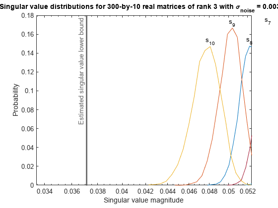
Plot the distribution of the singular values over all simulation runs. The distributions of the largest singular values correspond to the signals that determine the rank of the matrix. The distributions of the smallest singular values correspond to the noise. The derivation of the estimated bound of the smallest singular value makes use of the random nature of the noise.
clf
fixed.example.plot.singularValueDistribution(m,n,rankA,...
    noiseStandardDeviation,singularValues,...
    estimatedSingularValueLowerBound,"real");
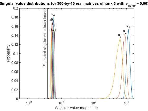
Zoom in to the smallest singular value to see that the estimated bound is close to it.
xlim([estimatedSingularValueLowerBound*0.9, max(singularValues(n,:))]);
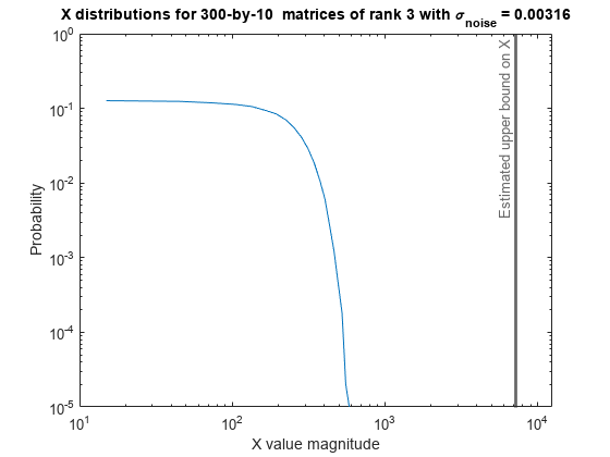
Estimate the largest value of the solution, X, and compare it to the largest value of X found during the simulation runs. The estimation is within an order of magnitude of the actual value, which is sufficient for estimating a fixed-point data type, because it is between 3 and 4 bits.
This example uses a limited number of simulation runs. With additional simulation runs, the actual largest value of X will approach the estimated largest value of X.
estimated_largest_X = fixed.realQlessQRMatrixSolveUpperBoundX(m,n,max_abs_B,noiseStandardDeviation)
estimated_largest_X =
7.2565e+03
actual_largest_X = max(abs(X_values),[],'all')actual_largest_X = 582.6761
Plot the distribution of X values and compare it to the estimated upper bound for X.
clf
fixed.example.plot.xValueDistribution(m,n,rankA,noiseStandardDeviation,...
    X_values,estimated_largest_X,"real normally distributed random");
Supporting Functions
The runSimulations function creates a series of random matrices and of a given size and rank, quantizes them according to the computed types, computes the QR decomposition of , and solves the equation . It returns the maximum values of , the singular values of , and the values of so their distributions can be plotted and compared to the bounds.
function [actualMaxR,singularValues,X_values] = runSimulations(m,n,p,rankA,max_abs_A,max_abs_B,...
        numSamples,noiseStandardDeviation,T)
    precisionBits = T.A.FractionLength;
    A_WordLength = T.A.WordLength;
    B_WordLength = T.B.WordLength;
    actualMaxR = zeros(1,numSamples);
    singularValues = zeros(n,numSamples);
    X_values = zeros(n,numSamples);
    for j = 1:numSamples
        A = max_abs_A*fixed.example.realRandomLowRankMatrix(m,n,rankA);
        % Adding random noise makes A non-singular.
        A = A + fixed.example.realNormalRandomArray(0,noiseStandardDeviation,m,n);
        A = quantizenumeric(A,1,A_WordLength,precisionBits);
        B = fixed.example.realUniformRandomArray(-max_abs_B,max_abs_B,n,p);
        B = quantizenumeric(B,1,B_WordLength,precisionBits);
        [~,R] = qr(A,0);
        X = R\(R'\B);
        actualMaxR(j) = max(abs(R(:)));
        singularValues(:,j) = svd(A);
        X_values(:,j) = X;
    end
end
References
Bryan, Thomas A., and Jenna L. Warren. "Systems and Methods for Design Parameter Selection." The MathWorks. US Patent 12,045,737 B2, issued July 23, 2024. European EP 3,944,105 A1. https://patents.google.com/patent/US12045737B2/en?oq=US+12%2c045%2c737+B2
Bryan, Thomas A., Jenna L. Warren, Shixin Zhuang, and Jessica Clayton. "Systems and Methods for Design Parameter Selection." The MathWorks. US Patent 12,008,344 B2, issued June 11, 2024. https://patents.google.com/patent/US12008344B2/en?oq=US+12%2c008%2c344+B2
Perform QR Factorization Using CORDIC. Derivation of the bound on growth when computing QR. MathWorks. 2010.
Zizhong Chen and Jack J. Dongarra. “Condition Numbers of Gaussian Random Matrices”. In: SIAM J. Matrix Anal. Appl. 27.3 (July 2005), pp. 603–620. issn: 0895-4798. doi: 10.1137/040616413. url: https://dx.doi.org/10.1137/040616413.
Bernard Widrow. “A Study of Rough Amplitude Quantization by Means of Nyquist Sampling Theory”. In: IRE Transactions on Circuit Theory 3.4 (Dec. 1956), pp. 266–276.
Bernard Widrow and István Kollár. Quantization Noise – Roundoff Error in Digital Computation, Signal Processing, Control, and Communications. Cambridge, UK: Cambridge University Press, 2008.
Gene H. Golub and Charles F. Van Loan. Matrix Computations. Second edition. Baltimore: Johns Hopkins University Press, 1989.
Suppress mlint warnings in this file.
%#ok<*NASGU>
%#ok<*ASGLU>
This example shows how to use the fixed.realQlessQRMatrixSolveFixedpointTypes function to analytically determine fixed-point types for the solution of the real least-squares matrix equation , where is an -by- matrix with , is -by-, and is -by-.
Fixed-point types for the solution of the matrix equation are well-bounded if the number of rows, , of are much greater than the number of columns, (i.e. ), and is full rank. If is not inherently full rank, then it can be made so by adding random noise. Random noise naturally occurs in physical systems, such as thermal noise in radar or communications systems. If , then the dynamic range of the system can be unbounded, for example in the scalar equation and , then can be arbitrarily large if is close to .
Define System Parameters
Define the matrix attributes and system parameters for this example.
m is the number of rows in matrix A. In a problem such as beamforming or direction finding, m corresponds to the number of samples that are integrated over.
m = 300;
n is the number of columns in matrix A and rows in matrices B and X. In a least-squares problem, m is greater than n, and usually m is much larger than n. In a problem such as beamforming or direction finding, n corresponds to the number of sensors.
n = 10;
p is the number of columns in matrices B and X. It corresponds to simultaneously solving a system with p right-hand sides.
p = 1;
In this example, set the rank of matrix A to be less than the number of columns. In a problem such as beamforming or direction finding, corresponds to the number of signals impinging on the sensor array.
rankA = 3;
precisionBits defines the number of bits of precision required for the matrix solve. Set this value according to system requirements.
precisionBits = 24;
In this example, real-valued matrices A and B are constructed such that the magnitude of their elements is less than or equal to one. Your own system requirements will define what those values are. If you don't know what they are, and A and B are fixed-point inputs to the system, then you can use the upperbound function to determine the upper bounds of the fixed-point types of A and B.
max_abs_A is an upper bound on the maximum magnitude element of A.
max_abs_A = 1;
max_abs_B is an upper bound on the maximum magnitude element of B.
max_abs_B = 1;
Thermal noise standard deviation is the square root of thermal noise power, which is a system parameter. A well-designed system has the quantization level lower than the thermal noise. Here, set thermalNoiseStandardDeviation to the equivalent of dB noise power.
thermalNoiseStandardDeviation = sqrt(10^(-50/10))
thermalNoiseStandardDeviation =
0.0032
The quantization noise standard deviation is a function of the required number of bits of precision. Use fixed.realQuantizationNoiseStandardDeviation to compute this. See that it is less than thermalNoiseStandardDeviation.
quantizationNoiseStandardDeviation = fixed.realQuantizationNoiseStandardDeviation(precisionBits)
quantizationNoiseStandardDeviation =
1.7206e-08
Compute Fixed-Point Types
In this example, assume that the designed system matrix does not have full rank (there are fewer signals of interest than number of columns of matrix ), and the measured system matrix has additive thermal noise that is larger than the quantization noise. The additive noise makes the measured matrix have full rank.
Set .
noiseStandardDeviation = thermalNoiseStandardDeviation;
Use fixed.realQlessQRMatrixSolveFixedpointTypes to compute fixed-point types.
T = fixed.realQlessQRMatrixSolveFixedpointTypes(m,n,max_abs_A,max_abs_B,...
    precisionBits,noiseStandardDeviation)
T = struct with fields:
A: [0×0 embedded.fi]
B: [0×0 embedded.fi]
X: [0×0 embedded.fi]
T.A is the type computed for transforming to in-place so that it does not overflow.
T.A
ans =

[]

          DataTypeMode: Fixed-point: binary point scaling
            Signedness: Signed
            WordLength: 31
        FractionLength: 24
T.B is the type computed for B so that it does not overflow.
T.B
ans =

[]

          DataTypeMode: Fixed-point: binary point scaling
            Signedness: Signed
            WordLength: 27
        FractionLength: 24
T.X is the type computed for the solution so that there is a low probability that it overflows.
T.X
ans =

[]

          DataTypeMode: Fixed-point: binary point scaling
            Signedness: Signed
            WordLength: 40
        FractionLength: 24
Use the Specified Types to Solve the Matrix Equation A'AX=B
Create random matrices A and B such that rankA=rank(A). Add random measurement noise to A which will make it become full rank.
rng('default');
[A,B] = fixed.example.realRandomQlessQRMatrices(m,n,p,rankA);
A = A + fixed.example.realNormalRandomArray(0,noiseStandardDeviation,m,n);
Cast the inputs to the types determined by fixed.realQlessQRMatrixSolveFixedpointTypes. Quantizing to fixed-point is equivalent to adding random noise [4,5].
A = cast(A,'like',T.A);
B = cast(B,'like',T.B);
Accelerate the fixed.qlessQRMatrixSolve function by using fiaccel to generate a MATLAB executable (MEX) function.
fiaccel fixed.qlessQRMatrixSolve -args {A,B,T.X} -o qlessQRMatrixSolve_mex
Specify output type T.X and compute fixed-point using the QR method.
X = qlessQRMatrixSolve_mex(A,B,T.X);
Compute the relative error to verify the accuracy of the output.
relative_error = norm(double(A'*A*X - B))/norm(double(B))
relative_error =
0.0624
Suppress mlint warnings in this file.
%#ok<*NASGU>
%#ok<*ASGLU>
This example shows how to use the fixed.realQlessQRMatrixSolveFixedpointTypes function to analytically determine fixed-point types for the solution of the real least-squares matrix equation
where is an -by- matrix with , is -by-, is -by-, , and is a regularization parameter.
Define System Parameters
Define the matrix attributes and system parameters for this example.
m is the number of rows in matrix A. In a problem such as beamforming or direction finding, m corresponds to the number of samples that are integrated over.
m = 300;
n is the number of columns in matrix A and rows in matrices B and X. In a least-squares problem, m is greater than n, and usually m is much larger than n. In a problem such as beamforming or direction finding, n corresponds to the number of sensors.
n = 10;
p is the number of columns in matrices B and X. It corresponds to simultaneously solving a system with p right-hand sides.
p = 1;
In this example, set the rank of matrix A to be less than the number of columns. In a problem such as beamforming or direction finding, corresponds to the number of signals impinging on the sensor array.
rankA = 3;
precisionBits defines the number of bits of precision required for the matrix solve. Set this value according to system requirements.
precisionBits = 32;
Small, positive values of the regularization parameter can improve the conditioning of the problem and reduce the variance of the estimates. While biased, the reduced variance of the estimate often results in a smaller mean squared error when compared to least-squares estimates.
regularizationParameter = 0.01;
In this example, real-valued matrices A and B are constructed such that the magnitude of their elements is less than or equal to one. Your own system requirements will define what those values are. If you don't know what they are, and A and B are fixed-point inputs to the system, then you can use the upperbound function to determine the upper bounds of the fixed-point types of A and B.
max_abs_A is an upper bound on the maximum magnitude element of A.
max_abs_A = 1;
max_abs_B is an upper bound on the maximum magnitude element of B.
max_abs_B = 1;
Thermal noise standard deviation is the square root of thermal noise power, which is a system parameter. A well-designed system has the quantization level lower than the thermal noise. Here, set thermalNoiseStandardDeviation to the equivalent of dB noise power.
thermalNoiseStandardDeviation = sqrt(10^(-50/10))
thermalNoiseStandardDeviation =
0.0032
The quantization noise standard deviation is a function of the required number of bits of precision. Use fixed.realQuantizationNoiseStandardDeviation to compute this. See that it is less than thermalNoiseStandardDeviation.
quantizationNoiseStandardDeviation = fixed.realQuantizationNoiseStandardDeviation(precisionBits)
quantizationNoiseStandardDeviation =
6.7212e-11
Compute Fixed-Point Types
In this example, assume that the designed system matrix does not have full rank (there are fewer signals of interest than number of columns of matrix ), and the measured system matrix has additive thermal noise that is larger than the quantization noise. The additive noise makes the measured matrix have full rank.
Set .
noiseStandardDeviation = thermalNoiseStandardDeviation;
Use the fixed.realQlessQRMatrixSolveFixedpointTypes function to compute fixed-point types.
T = fixed.realQlessQRMatrixSolveFixedpointTypes(m,n,max_abs_A,max_abs_B,...
    precisionBits,noiseStandardDeviation,[],regularizationParameter)
T = struct with fields:
A: [0×0 embedded.fi]
B: [0×0 embedded.fi]
X: [0×0 embedded.fi]
T.A is the type computed for transforming to in-place so that it does not overflow.
T.A
ans =

[]

          DataTypeMode: Fixed-point: binary point scaling
            Signedness: Signed
            WordLength: 39
        FractionLength: 32
T.B is the type computed for B so that it does not overflow.
T.B
ans =

[]

          DataTypeMode: Fixed-point: binary point scaling
            Signedness: Signed
            WordLength: 35
        FractionLength: 32
T.X is the type computed for the solution so that there is a low probability that it overflows.
T.X
ans =

[]

          DataTypeMode: Fixed-point: binary point scaling
            Signedness: Signed
            WordLength: 48
        FractionLength: 32
Use the Specified Types to Solve the Matrix Equation
Create random matrices A and B such that rankA=rank(A). Add random measurement noise to A which will make it become full rank.
rng('default');
[A,B] = fixed.example.realRandomQlessQRMatrices(m,n,p,rankA);
A = A + fixed.example.realNormalRandomArray(0,noiseStandardDeviation,m,n);
Cast the inputs to the types determined by fixed.realQlessQRMatrixSolveFixedpointTypes. Quantizing to fixed-point is equivalent to adding random noise.
A = cast(A,'like',T.A);
B = cast(B,'like',T.B);
Accelerate the fixed.qlessQRMatrixSolve function by using fiaccel to generate a MATLAB® executable (MEX) function.
fiaccel fixed.qlessQRMatrixSolve -args {A,B,T.X,[],regularizationParameter} -o qlessQRMatrixSolve_mex
Specify output type T.X and compute fixed-point using the QR method.
X = qlessQRMatrixSolve_mex(A,B,T.X,[],regularizationParameter);
Verify the Accuracy of the Output
Verify that the relative error between the fixed-point output and builtin MATLAB in double-precision floating-point is small.
A_lambda = double([regularizationParameter*eye(n);A]);
X_double = (A_lambda'*A_lambda)\double(B);
relativeError = norm(X_double - double(X))/norm(X_double)
relativeError =
1.0344e-05
Suppress mlint warnings in this file.
%#ok<*NASGU>
%#ok<*ASGLU>
Input Arguments
Output Arguments
Tips
Use fixed.realQlessQRMatrixSolveFixedpointTypes to compute
fixed-point types for the inputs of these functions and blocks.
Algorithms
The fixed-point type for A is computed using fixed.qlessqrFixedpointTypes. The required number of integer bits to prevent
overflow is derived from the following bound on the growth of R [1]. The
required number of integer bits is added to the number of bits of precision,
precisionBits, of the input, plus one for the sign bit, plus one bit
for intermediate CORDIC gain of approximately 1.6468 [2].
The elements of R are bounded in magnitude by
Matrix B is not transformed, so it does not need any additional growth bits.
The elements of X=R\(R'\B) are bounded in magnitude by
Computing the singular value decomposition to derive the above bound on
X is more computationally intensive than the entire matrix solve, so the
fixed.realSingularValueLowerBound function is used to estimate a bound on
min(svd(A)).
References
[2] Voler, Jack E. "The CORDIC Trigonometric Computing Technique." IRE Transactions on Electronic Computers EC-8 (1959): 330-334.