cordicsqrt

CORDIC-based approximation of square root

Syntax

y=cordicsqrt(u)

y=cordicsqrt(u, niters)

y=cordicsqrt(___, 'ScaleOutput', B)

Description

y=cordicsqrt(u) computes the square root of u using a CORDIC algorithm implementation.

y=cordicsqrt(u, niters) computes the square root of u by performing niters iterations of the CORDIC algorithm.

y=cordicsqrt(___, 'ScaleOutput', B) scales the output depending on the Boolean value of B.

Examples

Calculate the CORDIC Square Root

Find the square root of fi object x using a CORDIC implementation.

x = fi(1.6,1,12);
y = cordicsqrt(x)

y = 
    1.2646

          DataTypeMode: Fixed-point: binary point scaling
            Signedness: Signed
            WordLength: 12
        FractionLength: 10

Because you did not specify niters, the function performs the maximum number of iterations, x.WordLength - 1.

Compute the difference between the results of the cordicsqrt function and the double-precision sqrt function.

err = abs(sqrt(double(x))-double(y))

err = 
1.0821e-04

Calculate the CORDIC Square Root with a Specified Number of Iterations

Compute the square root of x with three iterations of the CORDIC kernel.

x = fi(1.6,1,12);
y = cordicsqrt(x,3)

y = 
    1.2646

          DataTypeMode: Fixed-point: binary point scaling
            Signedness: Signed
            WordLength: 12
        FractionLength: 10

Compute the difference between the results of the cordicsqrt function and the double-precision sqrt function.

err = abs(sqrt(double(x))-double(y))

err = 
1.0821e-04

Calculate the CORDIC Square Root Without Scaling the Output

x = fi(1.6,1,12);
y = cordicsqrt(x, 'ScaleOutput', 0)

y = 
    1.0479

          DataTypeMode: Fixed-point: binary point scaling
            Signedness: Signed
            WordLength: 12
        FractionLength: 10

The output, y, was not scaled by the inverse CORDIC gain factor.

Compare Results of cordicsqrt and sqrt Functions

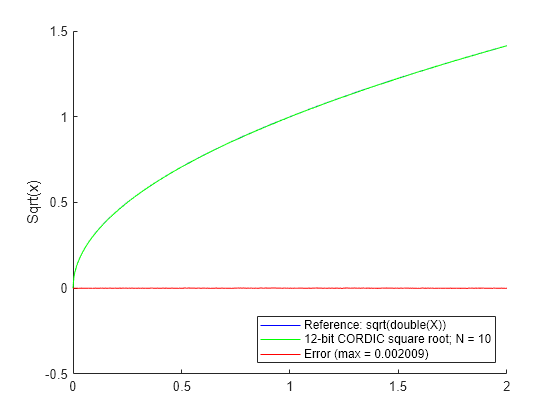
Compare the results produced by 10 iterations of the cordicsqrt algorithm to the results of the double-precision sqrt function.

Create 500 points in the interval [0, 2).

stepSize = 2/500;
XDbl = 0:stepSize:2;

Set the fixed-point type to be a signed 12-bit fixed-point type. Use the sqrt function with a double-precision input as reference.

XFxp = fi(XDbl,1,12);
sqrtXRef = sqrt(double(XFxp));

Set the number of CORDIC iterations to 10.

niters = 10;

Compare the fixed-point CORDIC results to the double-precision sqrt function.

cdcSqrtX  = cordicsqrt(XFxp,  niters);
errCdcRef = sqrtXRef - double(cdcSqrtX);

Plot the results.

figure
hold on
axis([0 2 -.5 1.5])
plot(XFxp, sqrtXRef,  'b')
plot(XFxp, cdcSqrtX,  'g')
plot(XFxp, errCdcRef, 'r')
ylabel('Sqrt(x)')
gca.XTick = 0:0.25:2;
gca.XTickLabel = {'0','0.25','0.5','0.75','1','1.25','1.5','1.75','2'};
gca.YTick = -.5:.25:1.5;
gca.YTickLabel = {'-0.5','-0.25','0','0.25','0.5','0.75','1','1.25','1.5'};
ref_str = 'Reference: sqrt(double(X))';
cdc_str = sprintf('12-bit CORDIC square root; N = %d', niters);
err_str = sprintf('Error (max = %f)', max(abs(errCdcRef)));
legend(ref_str, cdc_str, err_str, 'Location', 'southeast')

Input Arguments

u — Data input array

scalar | vector | matrix | multidimensional array

Data input array, specified as a positive scalar, vector, matrix, or multidimensional array of fixed-point or built-in data types. When the input array contains values between 0.5 and 2, the algorithm is most accurate. A pre- and post-normalization process is performed on input values outside of this range. For more information on this process, see Pre- and Post-Normalization.

Data Types: fi|single | double | int8 | int16 | int32 | int64 | uint8 | uint16 | uint32 | uint64

niters — Number of iterations

scalar

The number of iterations that the CORDIC algorithm performs, specified as a positive, integer-valued scalar. If you do not specify niters, the algorithm uses a default value. For fixed-point inputs, the default value of niters is u.WordLength - 1. For floating-point inputs, the default value of niters is 52 for double precision; 23 for single precision.

Data Types: fi|single | double | int8 | int16 | int32 | int64 | uint8 | uint16 | uint32 | uint64

ScaleOutput — Whether to scale the output

true (default) | false

Boolean value that specifies whether to scale the output by the inverse CORDIC gain factor. If you set ScaleOutput to true or 1, the output values are multiplied by a constant, which incurs extra computations. If you set ScaleOutput to false or 0, the output is not scaled.

Data Types: logical

Output Arguments

y — Output array

scalar | vector | matrix | multidimensional array

Output array, returned as a scalar, vector, matrix, or multidimensional array.

Algorithms

CORDIC

CORDIC is an acronym for COordinate Rotation DIgital Computer. The Givens rotation-based CORDIC algorithm is one of the most hardware-efficient algorithms available because it requires only iterative shift-add operations (see References). The CORDIC algorithm eliminates the need for explicit multipliers. Using CORDIC, you can calculate various functions such as sine, cosine, arcsine, arccosine, arctangent, and vector magnitude. You can also use this algorithm for divide, square root, hyperbolic, and logarithmic functions.

The precision of the CORDIC algorithm is a function of the data type used and the maximum shift value or number of iterations of the CORDIC kernel. Using a data type with a larger word length and performing more iterations of the CORDIC algorithm can reduce the numeric error of the result. However, doing so also increases the latency of the computation and the utilizes more hardware resources. For more information, see How to Set CORDIC Input Word Length and Maximum Shift Value to Achieve Desired Precision.

Signal Flow Diagrams

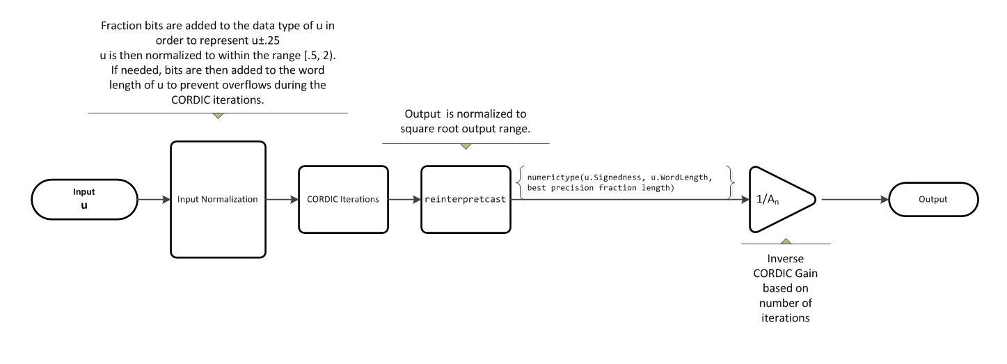
For further details on the pre- and post-normalization process, see Pre- and Post-Normalization.

CORDIC Hyperbolic Kernel

X is initialized to u'+.25, and Y is initialized to u'-.25, where u' is the normalized function input.

With repeated iterations of the CORDIC hyperbolic kernel, X approaches $$A_N\sqrt{u\text{'}}$$, where A_N represents the CORDIC gain. Y approaches 0.

Pre- and Post-Normalization

For input values outside of the range of [0.5, 2) a pre- and post-normalization process occurs. This process performs bit-shifts on the input array before passing it to the CORDIC kernel. The result is then shifted back into the correct output range during the post-normalization stage. For more details on this process, see Compute Square Root Using CORDIC.

fimath Propagation Rules

CORDIC functions discard any local fimath attached to the input.

The CORDIC functions use their own internal fimath when performing calculations:

• OverflowAction—Wrap

• RoundingMethod—Floor

The output has no attached fimath.

References

[1] Volder, Jack E. “The CORDIC Trigonometric Computing Technique.” IRE Transactions on Electronic Computers. EC-8, no. 3 (Sept. 1959): 330–334.

[2] Andraka, Ray. “A Survey of CORDIC Algorithm for FPGA Based Computers.” In Proceedings of the 1998 ACM/SIGDA Sixth International Symposium on Field Programmable Gate Arrays, 191–200. https://dl.acm.org/doi/10.1145/275107.275139.

[3] Walther, J.S. “A Unified Algorithm for Elementary Functions.” In Proceedings of the May 18-20, 1971 Spring Joint Computer Conference, 379–386. https://dl.acm.org/doi/10.1145/1478786.1478840.

[4] Schelin, Charles W. “Calculator Function Approximation.” The American Mathematical Monthly, no. 5 (May 1983): 317–325. https://doi.org/10.2307/2975781.

Extended Capabilities

C/C++ Code Generation

Generate C and C++ code using MATLAB® Coder™.

Usage notes and limitations:

• Variable-size signals are not supported.

• The number of iterations the CORDIC algorithm performs, niters, must be a constant.

HDL Code Generation

Generate VHDL, Verilog and SystemVerilog code for FPGA and ASIC designs using HDL Coder™.

The cordicsqrt function also supports MATLAB^® to High-Level Synthesis (HLS) code generation.

Version History

Introduced in R2014a