Pricing Asian Options
This example shows how to price a European Asian option using six methods in the Financial Instruments Toolbox™. This example demonstrates four closed form approximations (Kemna-Vorst, Levy, Turnbull-Wakeman, and Haug-Haug-Margrabe), a lattice model (Cox-Ross-Rubinstein), and Monte Carlo simulation. All these methods involve some tradeoffs between numerical accuracy and computational efficiency. This example also demonstrates how variations in spot prices, volatility, and strike prices affect option prices on European Vanilla and Asian options.
Overview of Asian Options
Asian options are securities with payoffs that depend on the average value of an underlying asset over a specific period of time. Underlying assets can be stocks, commodities, or financial indices.
Two types of Asian options are found in the market: average price options and average strike options. Average price options have a fixed strike value and the average used is the asset price. Average strike options have a strike equal to the average value of the underlying asset.
The payoff at maturity of an average price European Asian option is:
for a call
for a put
The payoff at maturity of an average strike European Asian option is:
for a call
for a put
where Savg is the average price of underlying asset, St is the price at maturity of underlying asset, and K is the strike price.
The average can be arithmetic or geometric.
Pricing Asian Options Using Closed Form Approximations
The Financial Instruments Toolbox™ supports four closed form approximations for European Average Price options. The Kemna-Vorst method is based on the geometric mean of the price of the underlying during the life of the option [1]. The Levy and Turnbull-Wakeman models provide a closed form pricing solution to continuous arithmetic averaging options [2,3]. The Haug-Haug-Margrabe approximation is used for pricing discrete arithmetic averaging options [4].
All the pricing functions asianbykv, asianbylevy, asianbytw, and asianbyhhm take an interest-rate term structure and stock structure as inputs.
Consider the following example:
% Create the RateSpec from the interest rate term structure.
StartDates = '12-March-2014';
EndDates = '12-March-2020';
Rates = 0.035;
Compounding = -1;
Basis = 1;

RateSpec = intenvset('ValuationDate', StartDates, 'StartDates', StartDates, ...
    'EndDates', EndDates, 'Rates', Rates, 'Compounding', ...
    Compounding, 'Basis', Basis);

% Define the StockSpec with the underlying asset information.
Sigma = 0.20;
AssetPrice = 100;

StockSpec = stockspec(Sigma, AssetPrice);

% Define the Asian option.
Settle = '12-March-2014';
ExerciseDates = '12-March-2015';
Strike = 90;
OptSpec = 'call';

% Kemna-Vorst closed form model
PriceKV = asianbykv(RateSpec, StockSpec, OptSpec, Strike, Settle,...
    ExerciseDates);

% Levy model approximation
PriceLevy = asianbylevy(RateSpec, StockSpec, OptSpec, Strike, Settle,...
    ExerciseDates);

% Turnbull-Wakeman approximation
PriceTW = asianbytw(RateSpec, StockSpec, OptSpec, Strike, Settle,...
    ExerciseDates);

% Haug-Haug-Margrabe approximation
PriceHHM = asianbyhhm(RateSpec, StockSpec, OptSpec, Strike, Settle,...
    ExerciseDates);

% Comparison of calculated prices for the geometric and arithmetic options
% using different closed form algorithms.
displayPricesClosedForm(PriceKV, PriceLevy, PriceTW, PriceHHM)
Comparison of Asian Arithmetic and Geometric Prices:

Kemna-Vorst:        11.862580
Levy:               12.164734
Turnbull-Wakeman:   12.164734
Haug-Haug-Margrabe: 12.108746
Computing Asian Options Prices Using the Cox-Ross-Rubinstein Model
In addition to closed form approximations, the Financial Instruments Toolbox™ supports pricing European Average Price options using CRR trees via the function asianbycrr.
The lattice pricing function asianbycrr takes an interest-rate tree ( CRRTree ) and stock structure as inputs. You can price the previous options by building a CRRTree using the interest-rate term structure and stock specification from the example above.
% Create the time specification of the tree.
NPeriods = 20;
TreeValuationDate = '12-March-2014';
TreeMaturity = '12-March-2024';
TimeSpec = crrtimespec(TreeValuationDate, TreeMaturity, NPeriods);

% Build the tree.
CRRTree =  crrtree(StockSpec, RateSpec, TimeSpec);

% Price the European Asian option using the CRR lattice model.
% The function 'asianbycrr' computes prices of arithmetic and geometric
% Asian options.
AvgType = {'arithmetic';'geometric'};
AmericanOpt = 0;
PriceCRR20 = asianbycrr(CRRTree, OptSpec, Strike, Settle, ExerciseDates, ...
                        AmericanOpt, AvgType);

% Increase the numbers of periods in the tree and compare results
NPeriods = 40;
TimeSpec = crrtimespec(TreeValuationDate, TreeMaturity, NPeriods);
CRRTree =  crrtree(StockSpec, RateSpec, TimeSpec);

PriceCRR40 = asianbycrr(CRRTree, OptSpec, Strike, Settle, ExerciseDates, ...
                        AmericanOpt, AvgType);

% Display prices
displayPricesCRR(PriceCRR20, PriceCRR40)
Asian Prices using the CRR lattice model:

PriceArithmetic(CRR20): 11.934380
PriceArithmetic(CRR40): 12.047243
PriceGeometric (CRR20): 11.620899
PriceGeometric (CRR40): 11.732037
The results above compare the findings from calculating both geometric and arithmetic Asian options, using CRR trees with 20 and 40 levels. As the number of levels increases, the results approach the closed form solutions.
Calculating Prices of Asian Options Using Monte Carlo Simulation
Another method to price European Average Price options with the Financial Instruments Toolbox™ is via Monte Carlo simulations.
The pricing function asianbyls takes an interest-rate term structure and stock structure as inputs. The output and execution time of the Monte Carlo simulation depends on the number of paths (NumTrials) and the number of time periods per path (NumPeriods).
You can price the same options of previous examples using Monte Carlo.
% Simulation Parameters
NumTrials = 500;
NumPeriods = 200;

% Price the arithmetic option
PriceAMC = asianbyls(RateSpec, StockSpec, OptSpec, Strike, Settle, ...
                     ExerciseDates,'NumTrials', NumTrials, ...
                     'NumPeriods', NumPeriods);

% Price the geometric option
PriceGMC = asianbyls(RateSpec, StockSpec, OptSpec, Strike, Settle,...
                     ExerciseDates,'NumTrials', NumTrials, ...
                     'NumPeriods', NumPeriods, 'AvgType', AvgType(2));

% Use the antithetic variates method to value the options
Antithetic = true;
PriceAMCAntithetic = asianbyls(RateSpec, StockSpec, OptSpec, Strike, Settle, ...
                    ExerciseDates,'NumTrials', NumTrials, 'NumPeriods', ...
                    NumPeriods, 'Antithetic', Antithetic);

PriceGMCAntithetic = asianbyls(RateSpec, StockSpec, OptSpec, Strike, Settle, ...
                    ExerciseDates,'NumTrials', NumTrials, 'NumPeriods', ...
                    NumPeriods, 'Antithetic', Antithetic,'AvgType', AvgType(2));

% Display prices
displayPricesMonteCarlo(PriceAMC, PriceAMCAntithetic, PriceGMC, PriceGMCAntithetic)
Asian Prices using Monte Carlo Method:

Arithmetic Asian
Standard Monte Carlo:           12.304046
Variate Antithetic Monte Carlo: 12.304046

Geometric Asian
Standard Monte Carlo:           12.048434
Variate Antithetic Monte Carlo: 12.048434
The use of variate antithetic accelerates the conversion process by reducing the variance.
You can create a plot to display the difference between the geometric Asian price using the Kemna-Vorst model, standard Monte Carlo, and antithetic Monte Carlo.
nTrials = [50:5:100 110:10:250 300:50:500 600:100:2500]';
PriceKVVector = PriceKV * ones(size(nTrials));
PriceGMCVector = nan(size(nTrials));
PriceGMCAntitheticVector = nan(size(nTrials));
TimeGMCAntitheticVector = nan(length(nTrials),1);
TimeGMCVector = nan(length(nTrials),1);
idx = 1;
for iNumTrials = nTrials'
    PriceGMCVector(idx) = asianbyls(RateSpec, StockSpec, OptSpec, Strike, Settle, ...
                        ExerciseDates,'NumTrials', iNumTrials, 'NumPeriods', ...
                        NumPeriods,'AvgType', AvgType(2));

    PriceGMCAntitheticVector(idx) = asianbyls(RateSpec, StockSpec, OptSpec, Strike, Settle, ...
                        ExerciseDates,'NumTrials', iNumTrials, 'NumPeriods', ...
                        NumPeriods, 'Antithetic', Antithetic,'AvgType', AvgType(2));
    idx = idx+1;
end

figure('menubar', 'none', 'numbertitle', 'off')
plot(nTrials, [PriceKVVector PriceGMCVector PriceGMCAntitheticVector]);
title 'Variance Reduction by Antithetic'
xlabel 'Number of Simulations'
ylabel 'Asian Option Price'
legend('Kemna-Vorst', 'Standard Monte Carlo', 'Variate Antithetic Monte Carlo ', 'location', 'northeast');

The graph above shows how oscillation in simulated price is reduced by using variate antithetic.
Compare Pricing Model Results
Prices calculated by the Monte Carlo method varies depending on the outcome of the simulations. Increase NumTrials and analyze the results.
NumTrials = 2000;

PriceAMCAntithetic2000 = asianbyls(RateSpec, StockSpec, OptSpec, Strike, Settle, ExerciseDates, ...
         'NumTrials', NumTrials, 'NumPeriods', NumPeriods, 'Antithetic', Antithetic);

PriceGMCAntithetic2000 = asianbyls(RateSpec, StockSpec, OptSpec, Strike, Settle, ...
                    ExerciseDates,'NumTrials', NumTrials, 'NumPeriods', ...
                    NumPeriods, 'Antithetic', Antithetic,'AvgType', AvgType(2));

% Comparison of calculated Asian call prices
displayComparisonAsianCallPrices(PriceLevy, PriceTW, PriceHHM, PriceCRR40, PriceAMCAntithetic, PriceAMCAntithetic2000, PriceKV, PriceGMCAntithetic, PriceGMCAntithetic2000)
Comparison of Asian call prices:

Arithmetic Asian
Levy:                     12.164734
Turnbull-Wakeman:         12.164734
Haug-Haug-Margrabe:       12.108746
Cox-Ross-Rubinstein:      12.047243
Monte Carlo(500 trials):  12.304046
Monte Carlo(2000 trials): 12.196848

Geometric Asian
Kemna-Vorst:              11.862580
Cox-Ross-Rubinstein:      11.732037
Monte Carlo(500 trials):  12.048434
Monte Carlo(2000 trials): 11.932017
The table above contrasts the results from closed approximation models against price simulations implemented via CRR trees and Monte Carlo.
Asian and Vanilla Call Options
Asian options are popular instruments since they tend to be less expensive than comparable Vanilla calls and puts. This is because the volatility in the average value of an underlier tends to be lower than the volatility of the value of the underlier itself.
The Financial Instruments Toolbox™ supports several algorithms for pricing vanilla options. Let us compare the price of Asian options against their Vanilla counterpart.
First, compute the price of a European Vanilla Option using the Black Scholes model.
PriceBLS = optstockbybls(RateSpec, StockSpec, Settle, ExerciseDates, ...
                         OptSpec, Strike);

% Comparison of calculated call prices.
displayComparisonVanillaAsian('Prices', PriceBLS, PriceKV, PriceLevy, PriceTW, PriceHHM)
Comparison of Vanilla and Asian Prices:

Vanilla BLS:              15.743809
Asian Kemna-Vorst:        11.862580
Asian Levy:               12.164734
Asian Turnbull-Wakeman:   12.164734
Asian Haug-Haug-Margrabe: 12.108746
Both geometric and arithmetic Asians price lower than their Vanilla counterpart.
You can analyze options prices at different levels of the underlying asset. Using the Financial Instruments Toolbox™, it is possible to observe the effect of different parameters on the price of the options. Consider for example, the effect of variations in the price of the underlying asset.
StockPrices = (50:5:150)';
PriceBLS = nan(size(StockPrices));
PriceKV = nan(size(StockPrices));
PriceLevy = nan(size(StockPrices));
PriceTW = nan(size(StockPrices));
PriceHHM = nan(size(StockPrices));
idx = 1;
for So = StockPrices'
    SP = stockspec(Sigma, So);
    PriceBLS(idx) = optstockbybls(RateSpec, SP, Settle, ExerciseDates, ...
                                  OptSpec, Strike);

    PriceKV(idx) = asianbykv(RateSpec, SP, OptSpec, Strike, Settle, ...
                             ExerciseDates);

    PriceLevy(idx) = asianbylevy(RateSpec, SP, OptSpec, Strike, Settle, ...
                                 ExerciseDates);

    PriceKV(idx) = asianbykv(RateSpec, SP, OptSpec, Strike, Settle, ...
                             ExerciseDates);

    PriceKV(idx) = asianbykv(RateSpec, SP, OptSpec, Strike, Settle, ...
                             ExerciseDates);

    idx = idx+1;
end

figure('menubar', 'none', 'numbertitle', 'off')
plot(StockPrices, [PriceBLS PriceKV PriceLevy PriceTW PriceHHM]);
xlabel 'Spot Price ($)'
ylabel 'Option Price ($)'
title 'Call Price Comparison'
legend('Vanilla', 'Geometric Asian', 'Continuous Arithmetic Asian (1)', 'Continuous Arithmetic Asian (2)', 'Discrete Arithmetic Asian', 'location', 'northwest');

It can be observed that the price of the Asian option is cheaper than the price of the Vanilla option.
Also, it is possible to observe the effect of changes in the volatility of the underlying asset. The table below shows what happens to Asian and Vanilla option prices when the constant volatility changes.
Call Option (ITM)
Strike = 90 AssetPrice = 100
-------------------------------------------------------------------------------------
Volatility Haug-Haug-Margrabe Turnbull-Wakeman Levy Kemna-Vorst BLS
10% 11.3946 11.3987 11.3987 11.3121 13.4343
20% 12.1087 12.1647 12.1647 11.8626 15.7438
30% 13.5374 13.6512 13.6512 13.0338 18.8770
40% 15.2823 15.4464 15.4464 14.4086 22.2507
A comparison of the calculated prices show that Asian options are less sensitive to volatility changes, since averaging reduces the volatility of the value of the underlying asset. Also, Asian options that use arithmetic average are more expensive than those that use geometric average.
Now, examine the effect of strike on option prices.
Strikes = (90:5:120)';
NStrike = length(Strikes);
PriceBLS = nan(size(Strikes));
PriceKV = nan(size(Strikes));
PriceLevy = nan(size(Strikes));
PriceTW = nan(size(Strikes));
PriceHHM = nan(size(Strikes));
idx = 1;
for ST = Strikes'
    SP = stockspec(Sigma, AssetPrice);
    PriceBLS(idx) = optstockbybls(RateSpec, SP, Settle, ExerciseDates, ...
                                  OptSpec, ST);

    PriceKV(idx) = asianbykv(RateSpec, SP, OptSpec, ST, Settle, ...
                             ExerciseDates);

    PriceLevy(idx) = asianbylevy(RateSpec, SP, OptSpec, ST, Settle, ...
                                 ExerciseDates);

    PriceTW(idx) = asianbytw(RateSpec, SP, OptSpec, ST, Settle, ...
                             ExerciseDates);

    PriceHHM(idx) = asianbyhhm(RateSpec, SP, OptSpec, ST, Settle, ...
                             ExerciseDates);

    idx = idx+1;
end

figure('menubar', 'none', 'numbertitle', 'off')
plot(Strikes, [PriceBLS PriceKV PriceLevy PriceTW PriceHHM]);
xlabel 'Strike Price ($)'
ylabel 'Option Price ($)'
title 'Effect of Strike on Option Prices'
legend('Vanilla', 'Geometric Asian', 'Continuous Arithmetic Asian (1)', 'Continuous Arithmetic Asian (2)', 'Discrete Arithmetic Asian', 'location', 'northeast');
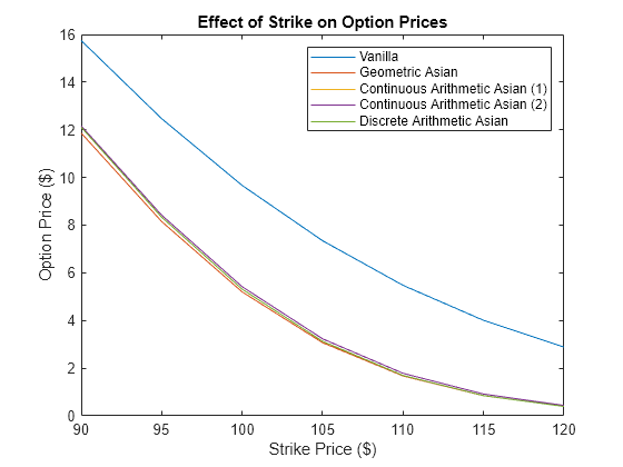
The figure above displays the option price with respect to strike price. Since call option value decreases as strike price increases, the Asian call curve is under the Vanilla call curve. It can be observed that the Asian call option is less expensive than the Vanilla call.
Hedging
Hedging is an insurance to minimize exposure to market movements on the value of a position or portfolio. As the underlying changes, the proportions of the instruments forming the portfolio may need to be adjusted to keep the sensitivities within the desired range. Delta measures the option price sensitivity to changes in the price of the underlying.
Assume that you have a portfolio of two options with the same strike and maturity. You can use the Financial Instruments Toolbox™ to compute Delta for the Vanilla and Average Price options.
OutSpec = 'Delta';

% Vanilla option using Black Scholes
DeltaBLS = optstocksensbybls(RateSpec, StockSpec, Settle, ExerciseDates, ...
                             OptSpec, Strike, 'OutSpec', OutSpec);

% Asian option using Kemna-Vorst method
DeltaKV = asiansensbykv(RateSpec, StockSpec, OptSpec, Strike, Settle, ...
                        ExerciseDates,  'OutSpec', OutSpec);

% Asian option using Levy model
DeltaLevy = asiansensbylevy(RateSpec, StockSpec, OptSpec, Strike, Settle, ...
                            ExerciseDates,  'OutSpec', OutSpec);

% Asian option using Turnbull-Wakeman model
DeltaTW = asiansensbytw(RateSpec, StockSpec, OptSpec, Strike, Settle, ...
                        ExerciseDates,  'OutSpec', OutSpec);

% Asian option using Haug-Haug-Margrabe model
DeltaHHM = asiansensbyhhm(RateSpec, StockSpec, OptSpec, Strike, Settle, ...
                        ExerciseDates,  'OutSpec', OutSpec);

% Delta Comparison
displayComparisonVanillaAsian('Delta', DeltaBLS, DeltaKV, DeltaLevy, DeltaTW, DeltaHHM)
Comparison of Vanilla and Asian Delta:

Vanilla BLS:              0.788666
Asian Kemna-Vorst:        0.844986
Asian Levy:               0.852806
Asian Turnbull-Wakeman:   0.852806
Asian Haug-Haug-Margrabe: 0.857864
The following graph demonstrates the behavior of Delta for the Vanilla and Asian options as a function of the underlying price.
StockPrices = (40:5:120)';
NStockPrices = length(StockPrices);
DeltaBLS = nan(size(StockPrices));
DeltaKV = nan(size(StockPrices));
DeltaLevy = nan(size(StockPrices));
DeltaTW = nan(size(StockPrices));
DeltaHHM = nan(size(StockPrices));

idx = 1;
for SPrices = StockPrices'
    SP = stockspec(Sigma, SPrices);
    DeltaBLS(idx) = optstocksensbybls(RateSpec, SP, Settle, ...
                    ExerciseDates, OptSpec, Strike, 'OutSpec', OutSpec);

    DeltaKV(idx) = asiansensbykv(RateSpec, SP, OptSpec, Strike, ...
                   Settle, ExerciseDates,'OutSpec', OutSpec);

    DeltaLevy(idx) = asiansensbylevy(RateSpec, SP, OptSpec, Strike, ...
                     Settle, ExerciseDates, 'OutSpec', OutSpec);

    DeltaTW(idx) = asiansensbytw(RateSpec, SP, OptSpec, Strike, ...
                   Settle, ExerciseDates,'OutSpec', OutSpec);

    DeltaHHM(idx) = asiansensbyhhm(RateSpec, SP, OptSpec, Strike, ...
                   Settle, ExerciseDates,'OutSpec', OutSpec);

    idx = idx+1;
end

figure('menubar', 'none', 'numbertitle', 'off')
plot(StockPrices, [DeltaBLS DeltaKV DeltaLevy DeltaTW DeltaHHM]);
xlabel 'Spot Price ($)'
ylabel 'Call Delta'
title 'Delta Comparison (Strike Price = $90)'
legend('Vanilla', 'Geometric Asian', 'Continuous Arithmetic Asian (1)', 'Continuous Arithmetic Asian (2)', 'Discrete Arithmetic Asian', 'location', 'northwest');
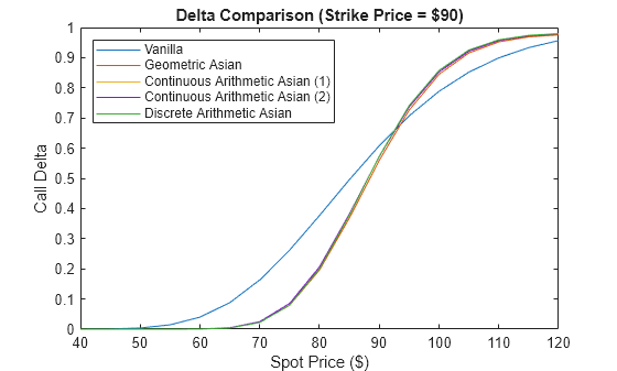
A Vanilla, or Asian, in the money (ITM) call option is more sensitive to price movements than an out of the money (OTM) option. If the asset price is deep in the money, then it is more likely to be exercised. The opposite occurs for an out of the money option. Asian delta is lower for out of the money options and is higher for in the money options than its Vanilla European counterpart. The geometric Asian delta is lower than the arithmetic Asian delta.
References
[1] Kemna, A. and Vorst, A. "A Pricing Method for Options Based on Average Asset Values." Journal of Banking and Finance. Vol. 14, 1990, pp. 113-129.
[2] Levy, E. "Pricing European Average Rate Currency Options." Journal of International Money and Finance. Vol. 11,1992, pp. 474-491.
[3] Turnbull, S. M., and Wakeman, L.M. "A Quick Algorithm for Pricing European Average Options." Journal of Financial and Quantitative Analysis. Vol. 26(3), 1991, pp. 377-389.
[4] Haug, E. G. The Complete Guide to Option Pricing Formulas. McGraw-Hill, New York, 2007.
Utility Functions
function displayPricesClosedForm(PriceKV, PriceLevy, PriceTW, PriceHHM)
fprintf('Comparison of Asian Arithmetic and Geometric Prices:\n');
fprintf('\n');
fprintf('Kemna-Vorst:        %f\n', PriceKV);
fprintf('Levy:               %f\n', PriceLevy);
fprintf('Turnbull-Wakeman:   %f\n', PriceTW);
fprintf('Haug-Haug-Margrabe: %f\n', PriceHHM);
end

function displayPricesCRR(PriceCRR20, PriceCRR40)
fprintf('Asian Prices using the CRR lattice model:\n');
fprintf('\n');
fprintf('PriceArithmetic(CRR20): %f\n', PriceCRR20(1));
fprintf('PriceArithmetic(CRR40): %f\n', PriceCRR40(1));
fprintf('PriceGeometric (CRR20): %f\n', PriceCRR20(2));
fprintf('PriceGeometric (CRR40): %f\n', PriceCRR40(2));
end

function displayPricesMonteCarlo(PriceAMC, PriceAMCAntithetic, PriceGMC, PriceGMCAntithetic)
fprintf('Asian Prices using Monte Carlo Method:\n');
fprintf('\n');
fprintf('Arithmetic Asian\n');
fprintf('Standard Monte Carlo:           %f\n', PriceAMC);
fprintf('Variate Antithetic Monte Carlo: %f\n\n', PriceAMCAntithetic);
fprintf('Geometric Asian\n');
fprintf('Standard Monte Carlo:           %f\n', PriceGMC);
fprintf('Variate Antithetic Monte Carlo: %f\n', PriceGMCAntithetic);
end

function displayComparisonAsianCallPrices(PriceLevy, PriceTW, PriceHHM, PriceCRR40, PriceAMCAntithetic, PriceAMCAntithetic2000, PriceKV, PriceGMCAntithetic, PriceGMCAntithetic2000)
fprintf('Comparison of Asian call prices:\n');
fprintf('\n');
fprintf('Arithmetic Asian\n');
fprintf('Levy:                     %f\n', PriceLevy);
fprintf('Turnbull-Wakeman:         %f\n', PriceTW);
fprintf('Haug-Haug-Margrabe:       %f\n', PriceHHM);
fprintf('Cox-Ross-Rubinstein:      %f\n', PriceCRR40(1));
fprintf('Monte Carlo(500 trials):  %f\n', PriceAMCAntithetic);
fprintf('Monte Carlo(2000 trials): %f\n', PriceAMCAntithetic2000);
fprintf('\n');
fprintf('Geometric Asian\n');
fprintf('Kemna-Vorst:              %f\n', PriceKV);
fprintf('Cox-Ross-Rubinstein:      %f\n', PriceCRR40(2));
fprintf('Monte Carlo(500 trials):  %f\n', PriceGMCAntithetic);
fprintf('Monte Carlo(2000 trials): %f\n', PriceGMCAntithetic2000);
end

function displayComparisonVanillaAsian(type, BLS, KV, Levy, TW, HHM)
fprintf('Comparison of Vanilla and Asian %s:\n', type);
fprintf('\n');
fprintf('Vanilla BLS:              %f\n', BLS);
fprintf('Asian Kemna-Vorst:        %f\n', KV);
fprintf('Asian Levy:               %f\n', Levy);
fprintf('Asian Turnbull-Wakeman:   %f\n', TW);
fprintf('Asian Haug-Haug-Margrabe: %f\n', HHM);
end
See Also
asianbykv | asiansensbykv | asianbylevy | asiansensbylevy | asianbyhhm | asiansensbyhhm | asianbytw | asiansensbytw | asianbyls | asiansensbyls | asianbystt | asianbyitt | asianbyeqp | asianbycrr
Topics
- Use Black-Scholes Model to Price Asian Options with Several Equity Pricers
- Supported Equity Derivative Functions
- Supported Energy Derivative Functions
- Mapping Financial Instruments Toolbox Functions for Equity, Commodity, FX Instrument Objects