Vanilla

Vanilla instrument object

Description

Create and price a Vanilla instrument object for one or more Vanilla instruments using this workflow:

1. Use fininstrument to create a Vanilla instrument object for one or more Vanilla instruments.

2. Use finmodel to specify a BlackScholes, Bachelier, Heston, Bates, Merton, RoughBergomi, RoughHeston, or Dupire model for the Vanilla instrument object.

3. Choose a pricing method.

   • When using a BlackScholes model, use finpricer to specify a FiniteDifference, BlackScholes, BjerksundStensland, RollGeskeWhaley, VannaVolga, AssetTree, or AssetMonteCarlo pricing method for one or more Vanilla instruments.

   • When using a Heston, Bates, or Merton model, use finpricer to specify a FiniteDifference, NumericalIntegration, FFT, or AssetMonteCarlo pricing method for one or more Vanilla instruments.

   • When using a Dupire model, use finpricer to specify a FiniteDifference pricing method for one or more Vanilla instruments.

   • When using a Bachelier model, use finpricer to specify an AssetMonteCarlo pricing method for one or more Vanilla instruments.

   • When using a RoughBergomi or RoughHeston model, use finpricer to specify a RoughVolMonteCarlo pricing method for one or more Vanilla instruments.

For more information on this workflow, see Get Started with Workflows Using Object-Based Framework for Pricing Financial Instruments.

For more information on the available models and pricing methods for a Vanilla instrument, see Choose Instruments, Models, and Pricers.

Creation

Syntax

VanillaObj = fininstrument(InstrumentType,'Strike',strike_value,'ExerciseDate',exercise_date)

VanillaObj = fininstrument(___,Name,Value)

Description

VanillaObj = fininstrument(InstrumentType,'Strike',strike_value,'ExerciseDate',exercise_date) creates a Vanilla object for one or more Vanilla instruments by specifying InstrumentType and sets the properties for the required name-value pair arguments Strike and ExerciseDate. For more information on a Vanilla instrument, see More About.

VanillaObj = fininstrument(___,Name,Value) sets optional properties using additional name-value pairs in addition to the required arguments in the previous syntax. For example, VanillaObj = fininstrument("Vanilla",'Strike',100,'ExerciseDate',datetime(2019,1,30),'OptionType',"put",'ExerciseStyle',"American",'Name',"vanilla_instrument") creates a Vanilla put option with an American exercise. You can specify multiple name-value pair arguments.

Input Arguments

InstrumentType — Instrument type

string with value "Vanilla" | string array with values of "Vanilla" | character vector with value 'Vanilla' | cell array of character vectors with values of 'Vanilla'

Instrument type, specified as a string with the value of "Vanilla", a character vector with the value of 'Vanilla', an NINST-by-1 string array with values of "Vanilla", or an NINST-by-1 cell array of character vectors with values of 'Vanilla'.

Data Types: char | cell | string

Name-Value Arguments

Specify required and optional pairs of arguments as Name1=Value1,...,NameN=ValueN, where Name is the argument name and Value is the corresponding value. Name-value arguments must appear after other arguments, but the order of the pairs does not matter.

Before R2021a, use commas to separate each name and value, and enclose Name in quotes.

Example: VanillaObj = fininstrument("Vanilla",'Strike',100,'ExerciseDate',datetime(2019,1,30),'OptionType',"put",'ExerciseStyle',"American",'Name',"vanilla_instrument")

Required Vanilla Name-Value Pair Arguments

Strike — Option strike price value

nonnegative numeric | nonnegative numeric vector

Option strike price value, specified as the comma-separated pair consisting of 'Strike' and a scalar nonnegative numeric value or an NINST-by-1 nonnegative numeric vector.

Note

When using a "Bermudan" ExerciseStyle with a FiniteDifference pricer, the Strike is a vector.

Data Types: double

ExerciseDate — Option exercise date

datetime array | string array | date character vector

Option exercise date, specified as the comma-separated pair consisting of 'ExerciseDate' and a scalar or an NINST-by-1 vector using a datetime array, string array, or date character vectors.

Note

For a European option, there is only one ExerciseDate on the option expiry date.

When using a "Bermudan" ExerciseStyle with a FiniteDifference pricer, the ExerciseDate is a vector.

To support existing code, Vanilla also accepts serial date numbers as inputs, but they are not recommended.

If you use date character vectors or strings, the format must be recognizable by datetime because the ExerciseDate property is stored as a datetime.

Optional Vanilla Name-Value Pair Arguments

OptionType — Option type

"call" (default) | string with value "call" or "put" | string array with values of "call" or "put" | character vector with value 'call' or 'put' | cell array of character vectors with values of 'call' or 'put'

Option type, specified as the comma-separated pair consisting of 'OptionType' and a scalar string or character vector or an NINST-by-1 cell array of character vectors or string array.

A call option gives the holder the right to buy the underlying asset at the strike price, while a put option gives the holder the right to sell the underlying asset at the strike price.

Note

When you use a RollGeskeWhaley pricer with a Vanilla option, OptionType must be 'call'.

Data Types: char | cell | string

ExerciseStyle — Option exercise style

"European" (default) | string with value "European", "American", or "Bermudan" | string array with values of "European", "American", or "Bermudan" | character vector with value 'European', 'American', or 'Bermudan' | cell array of character vectors with values of 'European', 'American', or 'Bermudan'

Option exercise style, specified as the comma-separated pair consisting of 'ExerciseStyle' and a scalar string or character vector or an NINST-by-1 cell array of character vectors or string array.

Note

• When you use a BlackScholes pricer with a Vanilla option, the 'American' option type is not supported.

• When you use a RollGeskeWhaley or a BjerksundStensland pricer with a Vanilla option, you must specify an 'American' option.

• When you use a NumericalIntegration pricer with a Bates, Merton, or Heston model for a Vanilla option, the ExerciseStyle must be 'European'.

• When you use a FFT pricer with a Bates, Merton, or Heston model for a Vanilla option, the ExerciseStyle must be 'European'.

• When you use an AssetMonteCarlo pricer with a BlackScholes, Bates, Merton, or Heston model for a Vanilla option, the ExerciseStyle can be 'American', 'European', or 'Bermudan'.

• When you use a FiniteDifference pricer with a BlackScholes, Bachelier, Dupire, Bates, Merton, or Heston model for a Vanilla option, the ExerciseStyle can be 'American', 'European', or 'Bermudan'.

For more information on ExerciseStyle, see Supported Exercise Styles.

Data Types: string | cell | char

Name — User-defined name for instrument

" " (default) | string | string array | character vector | cell array of character vectors

User-defined name for one of more instruments, specified as the comma-separated pair consisting of 'Name' and a scalar string or character vector or an NINST-by-1 cell array of character vectors or string array.

Data Types: char | cell | string

Output Arguments

VanillaObj — Vanilla instrument

Vanilla object

Vanilla instrument, returned as a Vanilla object.

Properties

Strike — Option strike price value

nonnegative numeric | nonnegative numeric vector

Option strike price value, returned as a scalar nonnegative numeric or an NINST-by-1 nonnegative numeric vector.

Data Types: double

ExerciseDate — Option exercise date

datetime | vector of datetimes

Option exercise date, returned as a scalar datetime or an NINST-by-1 vector of datetimes.

Data Types: datetime

OptionType — Option type

"call" (default) | string with value "call" or "put" | string array with values of "call" or "put"

Option type, returned as a scalar string or an NINST-by-1 string array with values of "call" or "put".

Data Types: string

ExerciseStyle — Option type

"European" (default) | string with value "European", "American", or "Bermudan" | string array with values of "European", "American", or "Bermudan"

Option exercise style, returned as a scalar string or an NINST-by-1 string array with values of "European", "American", or "Bermudan".

Data Types: string

Name — User-defined name for instrument

" " (default) | string | string array

User-defined name for the instrument, returned as a scalar string or an NINST-by-1 string array.

Data Types: string

Object Functions

setExercisePolicy

Set exercise policy for FixedBondOption, FloatBondOption, or Vanilla instrument

Examples

Price Vanilla Instrument Using BlackScholes Model and BlackScholes Pricer

This example shows the workflow to price a Vanilla instrument when you use a BlackScholes model and a BlackScholes pricing method.

Create Vanilla Instrument Object

Use fininstrument to create a Vanilla instrument object.

VanillaOpt = fininstrument("Vanilla",'ExerciseDate',datetime(2018,5,1),'Strike',29,'OptionType',"put",'ExerciseStyle',"european",'Name',"vanilla_option")

VanillaOpt = 
  Vanilla with properties:

       OptionType: "put"
    ExerciseStyle: "european"
     ExerciseDate: 01-May-2018
           Strike: 29
             Name: "vanilla_option"

Create BlackScholes Model Object

Use finmodel to create a BlackScholes model object.

BlackScholesModel = finmodel("BlackScholes",'Volatility',0.25)

BlackScholesModel = 
  BlackScholes with properties:

     Volatility: 0.2500
    Correlation: 1

Create ratecurve Object

Create a flat ratecurve object using ratecurve.

Settle = datetime(2018,1,1);
Maturity = datetime(2019,1,1);
Rate = 0.05;
myRC = ratecurve('zero',Settle,Maturity,Rate,'Basis',1)

myRC = 
  ratecurve with properties:

                 Type: "zero"
          Compounding: -1
                Basis: 1
                Dates: 01-Jan-2019
                Rates: 0.0500
               Settle: 01-Jan-2018
         InterpMethod: "linear"
    ShortExtrapMethod: "next"
     LongExtrapMethod: "previous"

Create BlackScholes Pricer Object

Use finpricer to create a BlackScholes pricer object and use the ratecurve object for the 'DiscountCurve' name-value pair argument.

outPricer = finpricer("analytic",'DiscountCurve',myRC,'Model',BlackScholesModel,'SpotPrice',30,'DividendValue',0.045)

outPricer = 
  BlackScholes with properties:

    DiscountCurve: [1×1 ratecurve]
            Model: [1×1 finmodel.BlackScholes]
        SpotPrice: 30
    DividendValue: 0.0450
     DividendType: "continuous"

Price Vanilla Instrument

Use price to compute the price and sensitivities for the Vanilla instrument.

[Price, outPR] = price(outPricer,VanillaOpt,["all"])

Price = 
1.2046

outPR = 
  priceresult with properties:

       Results: [1×7 table]
    PricerData: []

outPR.Results

ans=1×7 table
    Price      Delta       Gamma      Lambda      Vega       Rho       Theta 
    ______    ________    ________    _______    ______    _______    _______

    1.2046    -0.36943    0.086269    -9.3396    6.4702    -4.0959    -2.3107

Price Multiple Vanilla Instruments Using BlackScholes Model and BlackScholes Pricer

This example shows the workflow to price multiple Vanilla instrument when you use a BlackScholes model and a BlackScholes pricing method.

Create Vanilla Instrument Object

Use fininstrument to create a Vanilla instrument object for three Vanilla instruments.

VanillaOpt = fininstrument("Vanilla",'ExerciseDate',datetime([2018,5,1 ; 2018,6,1 ; 2018,7,1]),'Strike',[29 ; 38 ; 70],'OptionType',"put",'ExerciseStyle',"european",'Name',"vanilla_option")

VanillaOpt=3×1 Vanilla array with properties:
    OptionType
    ExerciseStyle
    ExerciseDate
    Strike
    Name

Create BlackScholes Model Object

Use finmodel to create a BlackScholes model object.

BlackScholesModel = finmodel("BlackScholes",'Volatility',0.25)

BlackScholesModel = 
  BlackScholes with properties:

     Volatility: 0.2500
    Correlation: 1

Create ratecurve Object

Create a flat ratecurve object using ratecurve.

Settle = datetime(2018,1,1);
Maturity = datetime(2019,1,1);
Rate = 0.05;
myRC = ratecurve('zero',Settle,Maturity,Rate,'Basis',1)

myRC = 
  ratecurve with properties:

                 Type: "zero"
          Compounding: -1
                Basis: 1
                Dates: 01-Jan-2019
                Rates: 0.0500
               Settle: 01-Jan-2018
         InterpMethod: "linear"
    ShortExtrapMethod: "next"
     LongExtrapMethod: "previous"

Create BlackScholes Pricer Object

Use finpricer to create a BlackScholes pricer object and use the ratecurve object for the 'DiscountCurve' name-value pair argument.

outPricer = finpricer("analytic",'DiscountCurve',myRC,'Model',BlackScholesModel,'SpotPrice',30,'DividendValue',0.045)

outPricer = 
  BlackScholes with properties:

    DiscountCurve: [1×1 ratecurve]
            Model: [1×1 finmodel.BlackScholes]
        SpotPrice: 30
    DividendValue: 0.0450
     DividendType: "continuous"

Price Vanilla Instruments

Use price to compute the prices and sensitivities for the Vanilla instruments.

[Price, outPR] = price(outPricer,VanillaOpt,["all"])

Price = 3×1

    1.2046
    7.9479
   38.9392

outPR=3×1 priceresult array with properties:
    Results
    PricerData

outPR.Results

ans=1×7 table
    Price      Delta       Gamma      Lambda      Vega       Rho       Theta 
    ______    ________    ________    _______    ______    _______    _______

    1.2046    -0.36943    0.086269    -9.3396    6.4702    -4.0959    -2.3107

ans=1×7 table
    Price      Delta       Gamma      Lambda      Vega       Rho       Theta 
    ______    ________    ________    _______    ______    _______    _______

    7.9479    -0.89786    0.031587    -3.4532    2.9612    -14.535    -0.3563

ans=1×7 table
    Price      Delta        Gamma        Lambda        Vega         Rho      Theta 
    ______    ________    __________    ________    __________    _______    ______

    38.939    -0.97775    1.2279e-06    -0.77043    0.00013814    -34.136    2.0936

Price Vanilla Instrument Using BlackScholes Model and AssetTree Pricer for LR Binomial Tree

This example shows the workflow to price a Vanilla instrument when you use a BlackScholes model and an AssetTree pricing method using a Leisen-Reimer (LR) binomial tree.

Create Vanilla Instrument Object

Use fininstrument to create a Vanilla instrument object.

VanillaOpt = fininstrument("Vanilla",'ExerciseDate',datetime(2018,5,1),'Strike',29,'OptionType',"put",'ExerciseStyle',"european",'Name',"vanilla_option")

VanillaOpt = 
  Vanilla with properties:

       OptionType: "put"
    ExerciseStyle: "european"
     ExerciseDate: 01-May-2018
           Strike: 29
             Name: "vanilla_option"

Create BlackScholes Model Object

Use finmodel to create a BlackScholes model object.

BlackScholesModel = finmodel("BlackScholes",'Volatility',0.25)

BlackScholesModel = 
  BlackScholes with properties:

     Volatility: 0.2500
    Correlation: 1

Create ratecurve Object

Create a flat ratecurve object using ratecurve.

Settle = datetime(2018,1,1);
Maturity = datetime(2019,1,1);
Rate = 0.05;
myRC = ratecurve('zero',Settle,Maturity,Rate,'Basis',1)

myRC = 
  ratecurve with properties:

                 Type: "zero"
          Compounding: -1
                Basis: 1
                Dates: 01-Jan-2019
                Rates: 0.0500
               Settle: 01-Jan-2018
         InterpMethod: "linear"
    ShortExtrapMethod: "next"
     LongExtrapMethod: "previous"

Create AssetTree Pricer Object

Use finpricer to create an AssetTree pricer object for a LR equity tree and use the ratecurve object for the 'DiscountCurve' name-value pair argument.

NumPeriods = 15;
LRPricer = finpricer("AssetTree",'DiscountCurve',myRC,'Model',BlackScholesModel,'SpotPrice',50,'PricingMethod',"LeisenReimer",'Maturity',datetime(2018,5,1),'NumPeriods',NumPeriods)

LRPricer = 
  LRTree with properties:

    InversionMethod: PP1
             Strike: 50
               Tree: [1×1 struct]
         NumPeriods: 15
              Model: [1×1 finmodel.BlackScholes]
      DiscountCurve: [1×1 ratecurve]
          SpotPrice: 50
       DividendType: "continuous"
      DividendValue: 0
          TreeDates: [09-Jan-2018    17-Jan-2018    25-Jan-2018    02-Feb-2018    10-Feb-2018    18-Feb-2018    26-Feb-2018    06-Mar-2018    14-Mar-2018    22-Mar-2018    30-Mar-2018    07-Apr-2018    15-Apr-2018    23-Apr-2018    01-May-2018]

LRPricer.Tree

ans = struct with fields:
    Probs: [2×15 double]
    ATree: {1×16 cell}
     dObs: [01-Jan-2018    09-Jan-2018    17-Jan-2018    25-Jan-2018    02-Feb-2018    10-Feb-2018    18-Feb-2018    26-Feb-2018    06-Mar-2018    14-Mar-2018    22-Mar-2018    30-Mar-2018    07-Apr-2018    15-Apr-2018    23-Apr-2018    01-May-2018]
     tObs: [0 0.0222 0.0444 0.0667 0.0889 0.1111 0.1333 0.1556 0.1778 0.2000 0.2222 0.2444 0.2667 0.2889 0.3111 0.3333]

Price Vanilla Instrument

Use price to compute the price and sensitivities for the Vanilla instrument.

[Price, outPR] = price(LRPricer,VanillaOpt,["all"])

Price = 
3.5022e-06

outPR = 
  priceresult with properties:

       Results: [1×7 table]
    PricerData: [1×1 struct]

outPR.Results

ans=1×7 table
      Price          Delta         Gamma         Vega       Lambda         Rho           Theta   
    __________    ___________    __________    _________    _______    ___________    ___________

    3.5022e-06    -1.9331e-06    1.1068e-06    0.0016243    -30.496    -3.6747e-05    -0.00060106

outPR.PricerData.PriceTree

ans = struct with fields:
     PTree: {1×16 cell}
    ExTree: {1×16 cell}
      tObs: [0 0.0222 0.0444 0.0667 0.0889 0.1111 0.1333 0.1556 0.1778 0.2000 0.2222 0.2444 0.2667 0.2889 0.3111 0.3333]
      dObs: [01-Jan-2018    09-Jan-2018    17-Jan-2018    25-Jan-2018    02-Feb-2018    10-Feb-2018    18-Feb-2018    26-Feb-2018    06-Mar-2018    14-Mar-2018    22-Mar-2018    30-Mar-2018    07-Apr-2018    15-Apr-2018    23-Apr-2018    01-May-2018]
     Probs: [2×15 double]

outPR.PricerData.PriceTree.ExTree

ans=1×16 cell array
    {[0]}    {[0 0]}    {[0 0 0]}    {[0 0 0 0]}    {[0 0 0 0 0]}    {[0 0 0 0 0 0]}    {[0 0 0 0 0 0 0]}    {[0 0 0 0 0 0 0 0]}    {[0 0 0 0 0 0 0 0 0]}    {[0 0 0 0 0 0 0 0 0 0]}    {[0 0 0 0 0 0 0 0 0 0 0]}    {[0 0 0 0 0 0 0 0 0 0 0 0]}    {[0 0 0 0 0 0 0 0 0 0 0 0 0]}    {[0 0 0 0 0 0 0 0 0 0 0 0 0 0]}    {[0 0 0 0 0 0 0 0 0 0 0 0 0 0 0]}    {[0 0 0 0 0 0 0 0 0 0 0 0 0 0 0 1]}

Price Vanilla Instrument Using BlackScholes Model and AssetTree Pricer for Standard Trinomial Tree

This example shows the workflow to price a Vanilla instrument when you use a BlackScholes model and an AssetTree pricing method using a Standard Trinomial (STT) tree.

Create Vanilla Instrument Object

Use fininstrument to create a Vanilla instrument object.

VanillaOpt = fininstrument("Vanilla",'ExerciseDate',datetime(2018,5,1),'Strike',29,'OptionType',"put",'ExerciseStyle',"european",'Name',"vanilla_option")

VanillaOpt = 
  Vanilla with properties:

       OptionType: "put"
    ExerciseStyle: "european"
     ExerciseDate: 01-May-2018
           Strike: 29
             Name: "vanilla_option"

Create BlackScholes Model Object

Use finmodel to create a BlackScholes model object.

BlackScholesModel = finmodel("BlackScholes",'Volatility',0.25)

BlackScholesModel = 
  BlackScholes with properties:

     Volatility: 0.2500
    Correlation: 1

Create ratecurve Object

Create a flat ratecurve object using ratecurve.

Settle = datetime(2018,1,1);
Maturity = datetime(2019,1,1);
Rate = 0.05;
myRC = ratecurve('zero',Settle,Maturity,Rate,'Basis',1)

myRC = 
  ratecurve with properties:

                 Type: "zero"
          Compounding: -1
                Basis: 1
                Dates: 01-Jan-2019
                Rates: 0.0500
               Settle: 01-Jan-2018
         InterpMethod: "linear"
    ShortExtrapMethod: "next"
     LongExtrapMethod: "previous"

Create AssetTree Pricer Object

Use finpricer to create an AssetTree pricer object for a Standard Trinomial (STT) equity tree and use the ratecurve object for the 'DiscountCurve' name-value pair argument.

NumPeriods = 15;
STTPricer = finpricer("AssetTree",'DiscountCurve',myRC,'Model',BlackScholesModel,'SpotPrice',50,'PricingMethod',"StandardTrinomial",'Maturity',datetime(2018,5,1),'NumPeriods',NumPeriods)

STTPricer = 
  STTree with properties:

             Tree: [1×1 struct]
       NumPeriods: 15
            Model: [1×1 finmodel.BlackScholes]
    DiscountCurve: [1×1 ratecurve]
        SpotPrice: 50
     DividendType: "continuous"
    DividendValue: 0
        TreeDates: [09-Jan-2018    17-Jan-2018    25-Jan-2018    02-Feb-2018    10-Feb-2018    18-Feb-2018    26-Feb-2018    06-Mar-2018    14-Mar-2018    22-Mar-2018    30-Mar-2018    07-Apr-2018    15-Apr-2018    23-Apr-2018    01-May-2018]

STTPricer.Tree

ans = struct with fields:
    ATree: {1×16 cell}
    Probs: {[3×1 double]  [3×3 double]  [3×5 double]  [3×7 double]  [3×9 double]  [3×11 double]  [3×13 double]  [3×15 double]  [3×17 double]  [3×19 double]  [3×21 double]  [3×23 double]  [3×25 double]  [3×27 double]  [3×29 double]}
     dObs: [01-Jan-2018    09-Jan-2018    17-Jan-2018    25-Jan-2018    02-Feb-2018    10-Feb-2018    18-Feb-2018    26-Feb-2018    06-Mar-2018    14-Mar-2018    22-Mar-2018    30-Mar-2018    07-Apr-2018    15-Apr-2018    23-Apr-2018    01-May-2018]
     tObs: [0 0.0222 0.0444 0.0667 0.0889 0.1111 0.1333 0.1556 0.1778 0.2000 0.2222 0.2444 0.2667 0.2889 0.3111 0.3333]

Price Vanilla Instrument

Use price to compute the price and sensitivities for the Vanilla instrument.

[Price, outPR] = price(STTPricer,VanillaOpt,["all"])

Price = 
6.3773e-05

outPR = 
  priceresult with properties:

       Results: [1×7 table]
    PricerData: [1×1 struct]

outPR.Results

ans=1×7 table
      Price          Delta         Gamma         Vega       Lambda         Rho          Theta  
    __________    ___________    __________    _________    _______    ___________    _________

    6.3773e-05    -9.1432e-06    1.2388e-06    0.0034421    -21.514    -0.00064994    -0.001188

outPR.PricerData.PriceTree

ans = struct with fields:
     PTree: {1×16 cell}
    ExTree: {1×16 cell}
      tObs: [0 0.0222 0.0444 0.0667 0.0889 0.1111 0.1333 0.1556 0.1778 0.2000 0.2222 0.2444 0.2667 0.2889 0.3111 0.3333]
      dObs: [01-Jan-2018    09-Jan-2018    17-Jan-2018    25-Jan-2018    02-Feb-2018    10-Feb-2018    18-Feb-2018    26-Feb-2018    06-Mar-2018    14-Mar-2018    22-Mar-2018    30-Mar-2018    07-Apr-2018    15-Apr-2018    23-Apr-2018    01-May-2018]
     Probs: {[3×1 double]  [3×3 double]  [3×5 double]  [3×7 double]  [3×9 double]  [3×11 double]  [3×13 double]  [3×15 double]  [3×17 double]  [3×19 double]  [3×21 double]  [3×23 double]  [3×25 double]  [3×27 double]  [3×29 double]}

outPR.PricerData.PriceTree.ExTree

ans=1×16 cell array
    {[0]}    {[0 0 0]}    {[0 0 0 0 0]}    {[0 0 0 0 0 0 0]}    {[0 0 0 0 0 0 0 0 0]}    {[0 0 0 0 0 0 0 0 0 0 0]}    {[0 0 0 0 0 0 0 0 0 0 0 0 0]}    {[0 0 0 0 0 0 0 0 0 0 0 0 0 0 0]}    {[0 0 0 0 0 0 0 0 0 0 0 0 0 0 0 0 0]}    {[0 0 0 0 0 0 0 0 0 0 0 0 0 0 0 0 0 0 0]}    {[0 0 0 0 0 0 0 0 0 0 0 0 0 0 0 0 0 0 0 0 0]}    {[0 0 0 0 0 0 0 0 0 0 0 0 0 0 0 0 0 0 0 0 0 0 0]}    {[0 0 0 0 0 0 0 0 0 0 0 0 0 0 0 0 0 0 0 0 0 0 0 0 0]}    {[0 0 0 0 0 0 0 0 0 0 0 0 0 0 0 0 0 0 0 0 0 0 0 0 0 0 0]}    {[0 0 0 0 0 0 0 0 0 0 0 0 0 0 0 0 0 0 0 0 0 0 0 0 0 0 0 0 0]}    {[0 0 0 0 0 0 0 0 0 0 0 0 0 0 0 0 0 0 0 0 0 0 0 0 1 1 1 1 1 1 1]}

Price American Option for Vanilla Instrument Using BlackScholes Model and RollGeskeWhaley Pricer

This example shows the workflow to price an American option for a Vanilla instrument when you use a BlackScholes model and a RollGeskeWhaley pricing method.

Create Vanilla Instrument Object

Use fininstrument to create a Vanilla instrument object.

VanillaOpt = fininstrument("Vanilla",'Strike',105,'ExerciseDate',datetime(2022,9,15),'OptionType',"call",'ExerciseStyle',"american",'Name',"vanilla_option")

VanillaOpt = 
  Vanilla with properties:

       OptionType: "call"
    ExerciseStyle: "american"
     ExerciseDate: 15-Sep-2022
           Strike: 105
             Name: "vanilla_option"

Create BlackScholes Model Object

Use finmodel to create a BlackScholes model object.

BlackScholesModel = finmodel("BlackScholes","Volatility",0.2)

BlackScholesModel = 
  BlackScholes with properties:

     Volatility: 0.2000
    Correlation: 1

Create ratecurve Object

Create a flat ratecurve object using ratecurve.

Settle = datetime(2018,9,15);
Maturity = datetime(2023,9,15);
Rate = 0.035;
myRC = ratecurve('zero',Settle,Maturity,Rate,'Basis',12)

myRC = 
  ratecurve with properties:

                 Type: "zero"
          Compounding: -1
                Basis: 12
                Dates: 15-Sep-2023
                Rates: 0.0350
               Settle: 15-Sep-2018
         InterpMethod: "linear"
    ShortExtrapMethod: "next"
     LongExtrapMethod: "previous"

Create RollGeskeWhaley Pricer Object

Use finpricer to create a RollGeskeWhaley pricer object and use the ratecurve object for the 'DiscountCurve' name-value pair argument.

outPricer = finpricer("analytic",'Model',BlackScholesModel,'DiscountCurve',myRC,'SpotPrice',100,'DividendValue',timetable(datetime(2021,6,15),0.25),'PricingMethod',"RollGeskeWhaley")

outPricer = 
  RollGeskeWhaley with properties:

    DiscountCurve: [1×1 ratecurve]
            Model: [1×1 finmodel.BlackScholes]
        SpotPrice: 100
    DividendValue: [1×1 timetable]
     DividendType: "cash"

Price Vanilla Instrument

Use price to compute the price and sensitivities for the Vanilla instrument.

[Price, outPR] = price(outPricer,VanillaOpt,["all"])

Price = 
19.9066

outPR = 
  priceresult with properties:

       Results: [1×7 table]
    PricerData: []

outPR.Results

ans=1×7 table
    Price      Delta       Gamma      Lambda     Vega      Theta      Rho  
    ______    _______    _________    ______    ______    _______    ______

    19.907    0.66568    0.0090971    3.344     72.804    -3.4537    186.68

Price a Vanilla Instrument for Foreign Exchange Using BlackScholes Model and BlackScholes Pricer

This example shows the workflow to price a Vanilla instrument for foreign exchange (FX) when you use a BlackScholes model and a BlackScholes pricing method. Assume that the current exchange rate is $0.52 and has a volatility of 12% per annum. The annualized continuously compounded foreign risk-free rate is 8% per annum.

Create Vanilla Instrument Object

Use fininstrument to create a Vanilla instrument object.

VanillaOpt = fininstrument("Vanilla",'ExerciseDate',datetime(2022,9,15),'Strike',.50,'OptionType',"put",'ExerciseStyle',"european",'Name',"vanilla_fx_option")

VanillaOpt = 
  Vanilla with properties:

       OptionType: "put"
    ExerciseStyle: "european"
     ExerciseDate: 15-Sep-2022
           Strike: 0.5000
             Name: "vanilla_fx_option"

Create BlackScholes Model Object

Use finmodel to create a BlackScholes model object.

Sigma = .12;
BlackScholesModel = finmodel("BlackScholes","Volatility",Sigma)

BlackScholesModel = 
  BlackScholes with properties:

     Volatility: 0.1200
    Correlation: 1

Create ratecurve Object

Create a flat ratecurve object using ratecurve.

Settle = datetime(2018,9,15);
Maturity = datetime(2023,9,15);
Rate = 0.035;
myRC = ratecurve('zero',Settle,Maturity,Rate,'Basis',12)

myRC = 
  ratecurve with properties:

                 Type: "zero"
          Compounding: -1
                Basis: 12
                Dates: 15-Sep-2023
                Rates: 0.0350
               Settle: 15-Sep-2018
         InterpMethod: "linear"
    ShortExtrapMethod: "next"
     LongExtrapMethod: "previous"

Create BlackScholes Pricer Object

Use finpricer to create a BlackScholes pricer object and use the ratecurve object for the 'DiscountCurve' name-value pair argument. When pricing currencies using a Vanilla instrument, the DividendType must be 'continuous' and DividendValue is the annualized risk-free interest rate in the foreign country.

ForeignRate = 0.08;
outPricer = finpricer("analytic",'DiscountCurve',myRC,'Model',BlackScholesModel,'SpotPrice',.52,'DividendType',"continuous",'DividendValue',ForeignRate)

outPricer = 
  BlackScholes with properties:

    DiscountCurve: [1×1 ratecurve]
            Model: [1×1 finmodel.BlackScholes]
        SpotPrice: 0.5200
    DividendValue: 0.0800
     DividendType: "continuous"

Price Vanilla FX Instrument

Use price to compute the price and sensitivities for the Vanilla FX instrument.

[Price, outPR] = price(outPricer,VanillaOpt,["all"])

Price = 
0.0738

outPR = 
  priceresult with properties:

       Results: [1×7 table]
    PricerData: []

outPR.Results

ans=1×7 table
     Price       Delta      Gamma     Lambda      Vega        Rho        Theta  
    ________    ________    ______    _______    _______    _______    _________

    0.073778    -0.49349    2.0818    -4.7899    0.27021    -1.3216    -0.013019

Price American Option for Vanilla Instrument Using BlackScholes Model and AssetMonteCarlo Pricer

This example shows the workflow to price an American option for a Vanilla instrument when you use a BlackScholes model and an AssetMonteCarlo pricing method.

Create Vanilla Instrument Object

Use fininstrument to create a Vanilla instrument object.

VanillaOpt = fininstrument("Vanilla",'Strike',105,'ExerciseDate',datetime(2022,9,15),'OptionType',"call",'ExerciseStyle',"american",'Name',"vanilla_option")

VanillaOpt = 
  Vanilla with properties:

       OptionType: "call"
    ExerciseStyle: "american"
     ExerciseDate: 15-Sep-2022
           Strike: 105
             Name: "vanilla_option"

Create BlackScholes Model Object

Use finmodel to create a BlackScholes model object.

BlackScholesModel = finmodel("BlackScholes","Volatility",0.2)

BlackScholesModel = 
  BlackScholes with properties:

     Volatility: 0.2000
    Correlation: 1

Create ratecurve Object

Create a flat ratecurve object using ratecurve.

Settle = datetime(2018,9,15);
Maturity = datetime(2023,9,15);
Rate = 0.035;
myRC = ratecurve('zero',Settle,Maturity,Rate,'Basis',12)

myRC = 
  ratecurve with properties:

                 Type: "zero"
          Compounding: -1
                Basis: 12
                Dates: 15-Sep-2023
                Rates: 0.0350
               Settle: 15-Sep-2018
         InterpMethod: "linear"
    ShortExtrapMethod: "next"
     LongExtrapMethod: "previous"

Create AssetMonteCarlo Pricer Object

Use finpricer to create an AssetMonteCarlo pricer object and use the ratecurve object for the 'DiscountCurve' name-value pair argument.

outPricer = finpricer("AssetMonteCarlo",'DiscountCurve',myRC,"Model",BlackScholesModel,'SpotPrice',150,'simulationDates',datetime(2022,9,15))

outPricer = 
  GBMMonteCarlo with properties:

           DiscountCurve: [1×1 ratecurve]
               SpotPrice: 150
         SimulationDates: 15-Sep-2022
               NumTrials: 1000
           RandomNumbers: []
                   Model: [1×1 finmodel.BlackScholes]
            DividendType: "continuous"
           DividendValue: 0
        MonteCarloMethod: "standard"
    BrownianMotionMethod: "standard"

Price Vanilla Instrument

Use price to compute the price and sensitivities for the Vanilla instrument.

[Price, outPR] = price(outPricer,VanillaOpt,["all"])

Price = 
61.2010

outPR = 
  priceresult with properties:

       Results: [1×7 table]
    PricerData: [1×1 struct]

outPR.Results

ans=1×7 table
    Price      Delta       Gamma      Lambda     Rho       Theta      Vega 
    ______    _______    _________    ______    ______    _______    ______

    61.201    0.93074    0.0027813    2.2812    313.95    -3.7909    41.626

Price American Option for Vanilla Instrument Using BlackScholes Model and AssetMonteCarlo Pricer with Quasi-Monte Carlo Simulation

This example shows the workflow to price an American option for a Vanilla instrument when you use a BlackScholes model and an AssetMonteCarlo pricing method with quasi-Monte Carlo simulation.

Create Vanilla Instrument Object

Use fininstrument to create a Vanilla instrument object.

VanillaOpt = fininstrument("Vanilla",'Strike',105,'ExerciseDate',datetime(2022,9,15),'OptionType',"call",'ExerciseStyle',"american",'Name',"vanilla_option")

VanillaOpt = 
  Vanilla with properties:

       OptionType: "call"
    ExerciseStyle: "american"
     ExerciseDate: 15-Sep-2022
           Strike: 105
             Name: "vanilla_option"

Create BlackScholes Model Object

Use finmodel to create a BlackScholes model object.

BlackScholesModel = finmodel("BlackScholes","Volatility",0.2)

BlackScholesModel = 
  BlackScholes with properties:

     Volatility: 0.2000
    Correlation: 1

Create ratecurve Object

Create a flat ratecurve object using ratecurve.

Settle = datetime(2018,9,15);
Maturity = datetime(2023,9,15);
Rate = 0.035;
myRC = ratecurve('zero',Settle,Maturity,Rate,'Basis',12)

myRC = 
  ratecurve with properties:

                 Type: "zero"
          Compounding: -1
                Basis: 12
                Dates: 15-Sep-2023
                Rates: 0.0350
               Settle: 15-Sep-2018
         InterpMethod: "linear"
    ShortExtrapMethod: "next"
     LongExtrapMethod: "previous"

Create AssetMonteCarlo Pricer Object

Use finpricer to create an AssetMonteCarlo pricer object and use the ratecurve object for the 'DiscountCurve' name-value argument and the name-value arguments for MonteCarloMethod and BrownianMotionMethod.

outPricer = finpricer("AssetMonteCarlo",'DiscountCurve',myRC,"Model",BlackScholesModel,'SpotPrice',150,'simulationDates',datetime(2022,9,15),'NumTrials',1e3, ...
                     'MonteCarloMethod',"quasi",'BrownianMotionMethod',"brownian-bridge")

outPricer = 
  GBMMonteCarlo with properties:

           DiscountCurve: [1×1 ratecurve]
               SpotPrice: 150
         SimulationDates: 15-Sep-2022
               NumTrials: 1000
           RandomNumbers: []
                   Model: [1×1 finmodel.BlackScholes]
            DividendType: "continuous"
           DividendValue: 0
        MonteCarloMethod: "quasi"
    BrownianMotionMethod: "brownian-bridge"

Price Vanilla Instrument

Use price to compute the price and sensitivities for the Vanilla instrument.

[Price, outPR] = price(outPricer,VanillaOpt,"all")

Price = 
60.7272

outPR = 
  priceresult with properties:

       Results: [1×7 table]
    PricerData: [1×1 struct]

outPR.Results

ans=1×7 table
    Price      Delta       Gamma      Lambda     Rho       Theta      Vega 
    ______    _______    _________    ______    ______    _______    ______

    60.727    0.92248    0.0024038    2.2786    310.66    -3.7073    39.466

Price American Option for Vanilla Instrument Using Heston Model and AssetMonteCarlo Pricer

This example shows the workflow to price an American option for a Vanilla instrument when you use a Heston model and an AssetMonteCarlo pricing method.

Create Vanilla Instrument Object

Use fininstrument to create a Vanilla instrument object.

VanillaOpt = fininstrument("Vanilla",'Strike',105,'ExerciseDate',datetime(2022,9,15),'OptionType',"call",'ExerciseStyle',"american",'Name',"vanilla_option")

VanillaOpt = 
  Vanilla with properties:

       OptionType: "call"
    ExerciseStyle: "american"
     ExerciseDate: 15-Sep-2022
           Strike: 105
             Name: "vanilla_option"

Create Heston Model Object

Use finmodel to create a Heston model object.

HestonModel = finmodel("Heston",'V0',0.032,'ThetaV',0.07,'Kappa',0.003,'SigmaV',0.02,'RhoSV',0.09)

HestonModel = 
  Heston with properties:

        V0: 0.0320
    ThetaV: 0.0700
     Kappa: 0.0030
    SigmaV: 0.0200
     RhoSV: 0.0900

Create ratecurve Object

Create a flat ratecurve object using ratecurve.

Settle = datetime(2018,9,15);
Maturity = datetime(2023,9,15);
Rate = 0.035;
myRC = ratecurve('zero',Settle,Maturity,Rate,'Basis',12)

myRC = 
  ratecurve with properties:

                 Type: "zero"
          Compounding: -1
                Basis: 12
                Dates: 15-Sep-2023
                Rates: 0.0350
               Settle: 15-Sep-2018
         InterpMethod: "linear"
    ShortExtrapMethod: "next"
     LongExtrapMethod: "previous"

Create AssetMonteCarlo Pricer Object

Use finpricer to create an AssetMonteCarlo pricer object and use the ratecurve object for the 'DiscountCurve' name-value pair argument.

outPricer = finpricer("AssetMonteCarlo",'DiscountCurve',myRC,"Model",HestonModel,'SpotPrice',150,'simulationDates',datetime(2022,9,15))

outPricer = 
  HestonMonteCarlo with properties:

           DiscountCurve: [1×1 ratecurve]
               SpotPrice: 150
         SimulationDates: 15-Sep-2022
               NumTrials: 1000
           RandomNumbers: []
                   Model: [1×1 finmodel.Heston]
            DividendType: "continuous"
           DividendValue: 0
        MonteCarloMethod: "standard"
    BrownianMotionMethod: "standard"

Price Vanilla Instrument

Use price to compute the price and sensitivities for the Vanilla instrument.

[Price, outPR] = price(outPricer,VanillaOpt,["all"])

Price = 
60.5637

outPR = 
  priceresult with properties:

       Results: [1×8 table]
    PricerData: [1×1 struct]

outPR.Results

ans=1×8 table
    Price      Delta       Gamma      Lambda     Rho       Theta      Vega     VegaLT 
    ______    _______    _________    ______    ______    _______    ______    _______

    60.564    0.94774    0.0011954    2.3473    326.36    -3.7126    35.272    0.31155

Price Bermudan Option for Vanilla Instrument Using BlackScholes Model and FiniteDifference Pricer

This example shows the workflow to price a Bermudan option for a Vanilla instrument when you use a BlackScholes model and a FiniteDifference pricing method.

Create Vanilla Instrument Object

Use fininstrument to create a Vanilla instrument object.

VanillaOpt = fininstrument("Vanilla",'Strike',[110,120],'ExerciseDate',[datetime(2022,9,15) , datetime(2023,9,15)],'OptionType',"call",'ExerciseStyle',"Bermudan",'Name',"vanilla_option")

VanillaOpt = 
  Vanilla with properties:

       OptionType: "call"
    ExerciseStyle: "bermudan"
     ExerciseDate: [15-Sep-2022    15-Sep-2023]
           Strike: [110 120]
             Name: "vanilla_option"

Create BlackScholes Model Object

Use finmodel to create a BlackScholes model object.

BlackScholesModel = finmodel("BlackScholes","Volatility",0.2)

BlackScholesModel = 
  BlackScholes with properties:

     Volatility: 0.2000
    Correlation: 1

Create ratecurve Object

Create a flat ratecurve object using ratecurve.

Settle = datetime(2018,9,15);
Maturity = datetime(2023,9,15);
Rate = 0.035;
myRC = ratecurve('zero',Settle,Maturity,Rate,'Basis',12)

myRC = 
  ratecurve with properties:

                 Type: "zero"
          Compounding: -1
                Basis: 12
                Dates: 15-Sep-2023
                Rates: 0.0350
               Settle: 15-Sep-2018
         InterpMethod: "linear"
    ShortExtrapMethod: "next"
     LongExtrapMethod: "previous"

Create FiniteDifference Pricer Object

Use finpricer to create a FiniteDifference pricer object and use the ratecurve object for the 'DiscountCurve' name-value pair argument.

outPricer = finpricer("FiniteDifference",'Model',BlackScholesModel,'DiscountCurve',myRC,'SpotPrice',100)

outPricer = 
  FiniteDifference with properties:

     DiscountCurve: [1×1 ratecurve]
             Model: [1×1 finmodel.BlackScholes]
         SpotPrice: 100
    GridProperties: [1×1 struct]
      DividendType: "continuous"
     DividendValue: 0

Price Vanilla Instrument

Use price to compute the price and sensitivities for the Vanilla instrument.

[Price, outPR] = price(outPricer,VanillaOpt,["all"])

Price = 
18.6797

outPR = 
  priceresult with properties:

       Results: [1×7 table]
    PricerData: [1×1 struct]

outPR.Results

ans=1×7 table
    Price     Delta       Gamma      Lambda     Theta      Rho       Vega 
    _____    _______    _________    ______    _______    ______    ______

    18.68    0.62163    0.0091406    3.3278    -3.3154    184.31    83.162

Price Vanilla Instrument Using Heston Model and Multiple Different Pricers

This example shows the workflow to price a Vanilla instrument when you use a Heston model and various pricing methods.

Create Vanilla Instrument Object

Use fininstrument to create a Vanilla instrument object.

Settle = datetime(2017,6,29);
Maturity = datemnth(Settle,6);
Strike = 80;
VanillaOpt = fininstrument('Vanilla','ExerciseDate',Maturity,'Strike',Strike,'Name',"vanilla_option")

VanillaOpt = 
  Vanilla with properties:

       OptionType: "call"
    ExerciseStyle: "european"
     ExerciseDate: 29-Dec-2017
           Strike: 80
             Name: "vanilla_option"

Create Heston Model Object

Use finmodel to create a Heston model object.

V0 = 0.04;
ThetaV = 0.05;
Kappa = 1.0;
SigmaV = 0.2;
RhoSV = -0.7;

HestonModel = finmodel("Heston",'V0',V0,'ThetaV',ThetaV,'Kappa',Kappa,'SigmaV',SigmaV,'RhoSV',RhoSV)

HestonModel = 
  Heston with properties:

        V0: 0.0400
    ThetaV: 0.0500
     Kappa: 1
    SigmaV: 0.2000
     RhoSV: -0.7000

Create ratecurve object

Create a ratecurve object using ratecurve.

Rate = 0.03;
ZeroCurve = ratecurve('zero',Settle,Maturity,Rate);

Create NumericalIntegration, FFT, and FiniteDifference Pricer Objects

Use finpricer to create a NumericalIntegration, FFT, and FiniteDifference pricer objects and use the ratecurve object for the 'DiscountCurve' name-value pair argument.

SpotPrice = 80;
Strike = 80;
DividendYield = 0.02;

NIPricer = finpricer("NumericalIntegration",'Model', HestonModel,'SpotPrice',SpotPrice,'DiscountCurve',ZeroCurve,'DividendValue',DividendYield)

NIPricer = 
  NumericalIntegration with properties:

                Model: [1×1 finmodel.Heston]
        DiscountCurve: [1×1 ratecurve]
            SpotPrice: 80
         DividendType: "continuous"
        DividendValue: 0.0200
               AbsTol: 1.0000e-10
               RelTol: 1.0000e-10
     IntegrationRange: [1.0000e-09 Inf]
    CharacteristicFcn: @characteristicFcnHeston
            Framework: "heston1993"
       VolRiskPremium: 0
           LittleTrap: 1

FFTPricer = finpricer("FFT",'Model',HestonModel, ...
    'SpotPrice',SpotPrice,'DiscountCurve',ZeroCurve, ...
    'DividendValue',DividendYield,'NumFFT',8192)

FFTPricer = 
  FFT with properties:

                    Model: [1×1 finmodel.Heston]
            DiscountCurve: [1×1 ratecurve]
                SpotPrice: 80
             DividendType: "continuous"
            DividendValue: 0.0200
                   NumFFT: 8192
    CharacteristicFcnStep: 0.0100
            LogStrikeStep: 0.0767
        CharacteristicFcn: @characteristicFcnHeston
            DampingFactor: 1.5000
               Quadrature: "simpson"
           VolRiskPremium: 0
               LittleTrap: 1

FDPricer = finpricer("FiniteDifference",'Model',HestonModel,'SpotPrice',SpotPrice,'DiscountCurve',ZeroCurve,'DividendValue',DividendYield)

FDPricer = 
  FiniteDifference with properties:

     DiscountCurve: [1×1 ratecurve]
             Model: [1×1 finmodel.Heston]
         SpotPrice: 80
    GridProperties: [1×1 struct]
      DividendType: "continuous"
     DividendValue: 0.0200

Price Vanilla Instrument

Use the following sensitivities when pricing the Vanilla instrument.

InpSensitivity = ["delta", "gamma", "theta", "rho", "vega", "vegalt"];

Use price to compute the price and sensitivities for the Vanilla instrument that uses the NumericalIntegration pricer.

[PriceNI,  outPR_NI]  = price(NIPricer,VanillaOpt,InpSensitivity)

PriceNI = 
4.7007

outPR_NI = 
  priceresult with properties:

       Results: [1×7 table]
    PricerData: []

Use price to compute the price and sensitivities for the Vanilla instrument that uses the FFT pricer.

[PriceFFT, outPR_FFT] = price(FFTPricer,VanillaOpt,InpSensitivity)

PriceFFT = 
4.7007

outPR_FFT = 
  priceresult with properties:

       Results: [1×7 table]
    PricerData: []

Use price to compute the price and sensitivities for the Vanilla instrument that uses the FiniteDifference pricer.

[PriceFD,  outPR_FD]  = price(FDPricer,VanillaOpt,InpSensitivity)

PriceFD = 
4.7003

outPR_FD = 
  priceresult with properties:

       Results: [1×7 table]
    PricerData: [1×1 struct]

Aggregate the price results.

[outPR_NI.Results;outPR_FFT.Results;outPR_FD.Results]

ans=3×7 table
    Price      Delta      Gamma       Theta      Rho       Vega     VegaLT
    ______    _______    ________    _______    ______    ______    ______

    4.7007    0.57747     0.03392    -4.8474    20.805    17.028    5.2394
    4.7007    0.57747     0.03392    -4.8474    20.805    17.028    5.2394
    4.7003    0.57722    0.035254    -4.8483    20.801    17.046    5.2422

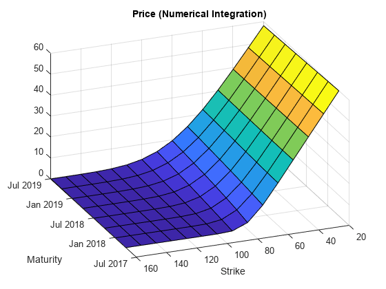
Compute Option Price Surfaces

Use the price function for the NumericalIntegration pricer and the price function for the FFT pricer to compute the prices for a range of Vanilla instruments.

Maturities = datemnth(Settle,(3:3:24)');
NumMaturities = length(Maturities);
Strikes = (20:10:160)';
NumStrikes = length(Strikes);

[Maturities_Full,Strikes_Full] = meshgrid(Maturities,Strikes);

NumInst = numel(Strikes_Full);
VanillaOptions(NumInst, 1) = fininstrument("vanilla", ...
    "ExerciseDate", Maturities_Full(1), "Strike", Strikes_Full(1));
for instidx=1:NumInst
    VanillaOptions(instidx) = fininstrument("vanilla", ...
        "ExerciseDate", Maturities_Full(instidx), "Strike", Strikes_Full(instidx));
end

Prices_NI = price(NIPricer, VanillaOptions);
Prices_FFT = price(FFTPricer, VanillaOptions);

figure;
surf(Maturities_Full,Strikes_Full,reshape(Prices_NI,[NumStrikes,NumMaturities]));
title('Price (Numerical Integration)');
view(-112,34);
xlabel('Maturity')
ylabel('Strike')

figure;
surf(Maturities_Full,Strikes_Full,reshape(Prices_FFT,[NumStrikes,NumMaturities]));
title('Price (FFT)');
view(-112,34);
xlabel('Maturity')
ylabel('Strike')

Price Vanilla Instrument Using RoughBergomi Model and RoughVolMonteCarlo Pricer

Since R2024a

This example shows the workflow to price a Vanilla instrument when you use a RoughBergomi model and a RoughVolMonteCarlo pricing method.

Create Vanilla Instrument Object

Use fininstrument to create a Vanilla instrument object.

VanillaOpt = fininstrument("Vanilla",'ExerciseDate',datetime(2019,1,30),'Strike',105,'ExerciseStyle',"european",'Name',"vanilla_option")

VanillaOpt = 
  Vanilla with properties:

       OptionType: "call"
    ExerciseStyle: "european"
     ExerciseDate: 30-Jan-2019
           Strike: 105
             Name: "vanilla_option"

Create RoughBergomi Model Object

Use finmodel to create a RoughBergomi model object.

RoughBergomiModel = finmodel("RoughBergomi",Alpha=-0.032,Xi=0.1,Eta=0.003,RhoSV=0.9)

RoughBergomiModel = 
  RoughBergomi with properties:

    Alpha: -0.0320
       Xi: 0.1000
      Eta: 0.0030
    RhoSV: 0.9000

Create ratecurve Object

Create a flat ratecurve object using ratecurve.

Settle = datetime(2018,9,15);
Maturity = datetime(2023,9,15);
Rate = 0.035;
myRC = ratecurve('zero',Settle,Maturity,Rate,'Basis',12)

myRC = 
  ratecurve with properties:

                 Type: "zero"
          Compounding: -1
                Basis: 12
                Dates: 15-Sep-2023
                Rates: 0.0350
               Settle: 15-Sep-2018
         InterpMethod: "linear"
    ShortExtrapMethod: "next"
     LongExtrapMethod: "previous"

Create RoughVolMonteCarlo Pricer Object

Use finpricer to create an RoughVolMonteCarlo pricer object and use the ratecurve object for the 'DiscountCurve' name-value pair argument.

outPricer = finpricer("RoughVolMonteCarlo",DiscountCurve=myRC,Model=RoughBergomiModel,SpotPrice=100,SimulationDates=datetime(2019,1,30))

outPricer = 
  RoughBergomiMonteCarlo with properties:

           DiscountCurve: [1×1 ratecurve]
               SpotPrice: 100
         SimulationDates: 30-Jan-2019
               NumTrials: 1000
           RandomNumbers: []
                   Model: [1×1 finmodel.RoughBergomi]
            DividendType: "continuous"
           DividendValue: 0
        MonteCarloMethod: "standard"
    BrownianMotionMethod: "standard"

Price Vanilla Instrument

Use price to compute the price and sensitivities for the Vanilla instrument.

[Price, outPR] = price(outPricer,VanillaOpt,"all")

Price = 
7.7862

outPR = 
  priceresult with properties:

       Results: [1×7 table]
    PricerData: [1×1 struct]

outPR.Results

ans=1×7 table
    Price      Delta      Gamma      Lambda     Rho      Theta      Vega 
    ______    _______    ________    ______    ______    ______    ______

    7.7862    0.50369    0.012632    6.469     15.947    1.0273    30.741

Price Vanilla Instrument Using RoughHeston Model and RoughVolMonteCarlo Pricer

Since R2024b

This example shows the workflow to price a Vanilla instrument when you use a RoughHeston model and a RoughVolMonteCarlo pricing method.

Create Vanilla Instrument Object

Use fininstrument to create a Vanilla instrument object.

VanillaOpt = fininstrument("Vanilla",'ExerciseDate',datetime(2019,1,30),'Strike',105,'ExerciseStyle',"european",'Name',"vanilla_option")

VanillaOpt = 
  Vanilla with properties:

       OptionType: "call"
    ExerciseStyle: "european"
     ExerciseDate: 30-Jan-2019
           Strike: 105
             Name: "vanilla_option"

Create RoughHeston Model Object

Use finmodel to create a RoughHeston model object.

RoughBergomiModel = finmodel("RoughHeston",V0=0.4,ThetaV=0.3,Kappa=0.2,SigmaV=0.1,Alpha=-0.02,RhoSV=0.3)

RoughBergomiModel = 
  RoughHeston with properties:

     Alpha: -0.0200
        V0: 0.4000
    ThetaV: 0.3000
     Kappa: 0.2000
    SigmaV: 0.1000
     RhoSV: 0.3000

Create ratecurve Object

Create a flat ratecurve object using ratecurve.

Settle = datetime(2018,9,15);
Maturity = datetime(2023,9,15);
Rate = 0.035;
myRC = ratecurve('zero',Settle,Maturity,Rate,'Basis',12)

myRC = 
  ratecurve with properties:

                 Type: "zero"
          Compounding: -1
                Basis: 12
                Dates: 15-Sep-2023
                Rates: 0.0350
               Settle: 15-Sep-2018
         InterpMethod: "linear"
    ShortExtrapMethod: "next"
     LongExtrapMethod: "previous"

Create RoughVolMonteCarlo Pricer Object

Use finpricer to create an RoughVolMonteCarlo pricer object and use the ratecurve object for the 'DiscountCurve' name-value argument.

outPricer = finpricer("RoughVolMonteCarlo",DiscountCurve=myRC,Model=RoughBergomiModel,SpotPrice=100,SimulationDates=datetime(2019,1,30))

outPricer = 
  RoughHestonMonteCarlo with properties:

           DiscountCurve: [1×1 ratecurve]
               SpotPrice: 100
         SimulationDates: 30-Jan-2019
               NumTrials: 1000
           RandomNumbers: []
                   Model: [1×1 finmodel.RoughHeston]
            DividendType: "continuous"
           DividendValue: 0
        MonteCarloMethod: "standard"
    BrownianMotionMethod: "standard"

Price Vanilla Instrument

Use price to compute the price and sensitivities for the Vanilla instrument.

[Price, outPR] = price(outPricer,VanillaOpt,"all")

Price = 
13.9392

outPR = 
  priceresult with properties:

       Results: [1×8 table]
    PricerData: [1×1 struct]

outPR.Results

ans=1×8 table
    Price      Delta      Gamma      Lambda     Rho       Theta      Vega     VegaLT
    ______    _______    ________    ______    ______    _______    ______    ______

    13.939    0.54193    0.011253    3.8878    15.143    -22.098    24.539      0   

More About

Vanilla Option

A vanilla option is a category of options that includes only the most standard components.

A vanilla option is based on an underlying asset, which can include stocks, bonds, commodities, currencies, or market indices. The value of the option is derived from the price movement of the underlying asset.

Vanilla options come in two forms: call options and put options. A call option gives the holder the right to buy the underlying asset at the strike price, while a put option gives the holder the right to sell the underlying asset at the strike price. The buyer of a vanilla option pays a premium to the seller or writer of the option in exchange for the rights provided by the option contract. The premium represents the cost of acquiring the option and is influenced by factors such as the price of the underlying asset, time to expiration, volatility, and prevailing market conditions.

The strike price, also known as the exercise price, is the predetermined price at which the underlying asset can be bought (in the case of a call option) or sold (in the case of a put option) if the option is exercised.

A vanilla option has an expiration date and straightforward strike price. After the expiration date, the option becomes void. American-style options and European-style options are both categorized as vanilla options.

The payoff for a vanilla option is as follows:

• For a call: $$\max (St-K,0)$$

• For a put: $$\max (K-St,0)$$

where:

St is the price of the underlying asset at time t.

K is the strike price.

For more information, see Vanilla Option.

Tips

After creating a Vanilla instrument object, you can use setExercisePolicy to change the size of the options. For example, if you have the following instrument:

VanillaOpt = fininstrument("Vanilla",'ExerciseDate',datetime(2021,5,1),'Strike',29,'OptionType',"put",'ExerciseStyle',"European")

To modify the Vanilla instrument's size by changing the ExerciseStyle from "European" to "American", use setExercisePolicy:

VanillaOpt = setExercisePolicy(VanillaOpt,[datetime(2021,1,1) datetime(2022,1,1)],100,'American')

Version History

Introduced in R2020a

R2024b: Support for RoughHeston model and RoughVolMonteCarlo pricer

The Vanilla instrument object supports pricing with a RoughHeston model and a RoughVolMonteCarlo pricing method.

R2024a: Support for RoughBergomi model and RoughVolMonteCarlo pricer

The Vanilla instrument object supports pricing with a RoughBergomi model and a RoughVolMonteCarlo pricing method.

R2022b: Serial date numbers not recommended

Although Vanilla supports serial date numbers, datetime values are recommended instead. The datetime data type provides flexible date and time formats, storage out to nanosecond precision, and properties to account for time zones and daylight saving time.

To convert serial date numbers or text to datetime values, use the datetime function. For example:

t = datetime(738427.656845093,"ConvertFrom","datenum");
y = year(t)

y =

        2021

There are no plans to remove support for serial date number inputs.