Main Content

interpolate

Brownian interpolation of stochastic differential equations (SDEs) for SDE, BM, GBM, CEV, CIR, HWV, Heston, SDEDDO, SDELD, or SDEMRD models

Description

[XT,T] = interpolate(MDL,Times,Paths) performs a Brownian interpolation into a user-specified time series array, based on a piecewise-constant Euler sampling approach.

example

[XT,T] = interpolate(___,Name,Value) adds optional name-value pair arguments.

example

Examples

collapse all

Many applications require knowledge of the state vector at intermediate sample times that are initially unavailable. One way to approximate these intermediate states is to perform a deterministic interpolation. However, deterministic interpolation techniques fail to capture the correct probability distribution at these intermediate times. Brownian (or stochastic) interpolation captures the correct joint distribution by sampling from a conditional Gaussian distribution. This sampling technique is sometimes referred to as a Brownian Bridge.

The default stochastic interpolation technique is designed to interpolate into an existing time series and ignore new interpolated states as additional information becomes available. This technique is the usual notion of interpolation, which is called Interpolation without refinement.

Alternatively, the interpolation technique may insert new interpolated states into the existing time series upon which subsequent interpolation is based, by that means refining information available at subsequent interpolation times. This technique is called interpolation with refinement.

Interpolation without refinement is a more traditional technique, and is most useful when the input series is closely spaced in time. In this situation, interpolation without refinement is a good technique for inferring data in the presence of missing information, but is inappropriate for extrapolation. Interpolation with refinement is more suitable when the input series is widely spaced in time, and is useful for extrapolation.

The stochastic interpolation method is available to any model. It is best illustrated, however, by way of a constant-parameter Brownian motion process. Consider a correlated, bivariate Brownian motion (BM) model of the form:

interpolate_refpageeq1.gif

Specify BM Model

Create a bm object to represent the bivariate model.

mu    = [0.3; 0.4];
sigma = [0.2 -0.1; 0.1 -0.2];
rho   = [1 0.5; 0.5 1];
obj   = bm(mu,sigma,'Correlation',rho);

Simulate Single Path from BM

Assuming that the drift (Mu) and diffusion (Sigma) parameters are annualized, simulate a single Monte Carlo trial of daily observations for one calendar year (250 trading days).

rng default  % Make output reproducible
dt    = 1/250;  % 1 trading day = 1/250 years
[X,T] = simulate(obj,250,'DeltaTime',dt);

Interpolate Into Simulated Time Series

Interpolate into the simulated time series with a Brownian bridge.

t = ((T(1) + dt/2):(dt/2):(T(end) - dt/2));
x = interpolate(obj,t,X,'Times',T);

Plot Simulated and Interpolated Values

Plot both the simulated and interpolated values.

plot(T,X(:,1),'.-r',T,X(:,2),'.-b')
grid on;
hold on;
plot(t,x(:,1),'or',t,x(:,2),'ob')
hold off;
xlabel('Time (Years)')
ylabel('State')
title('Bi-Variate Brownian Motion: \rho = 0.5')
axis([0.4999 0.6001 0.25 0.4])

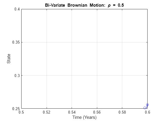
Figure contains an axes object. The axes object with title Bi-Variate blank Brownian blank Motion: blank rho blank = blank 0 . 5, xlabel Time (Years), ylabel State contains 4 objects of type line. One or more of the lines displays its values using only markers

In this plot:

  • The solid red and blue dots indicate the simulated states of the bivariate model.

  • The straight lines that connect the solid dots indicate intermediate states that would be obtained from a deterministic linear interpolation.

  • Open circles indicate interpolated states.

  • Open circles associated with every other interpolated state encircle solid dots associated with the corresponding simulated state. However, interpolated states at the midpoint of each time increment typically deviate from the straight line connecting each solid dot.

You can gain additional insight into the behavior of stochastic interpolation by regarding a Brownian bridge as a Monte Carlo simulation of a conditional Gaussian distribution. This example examines the behavior of a Brownian bridge over a single time increment.

Create Subintervals

Divide a single time increment of length dt into 10 subintervals.

mu    = [0.3; 0.4];
sigma = [0.2 -0.1; 0.1 -0.2];
rho   = [1 0.5; 0.5 1];
obj   = bm(mu,sigma,'Correlation',rho);

rng default; % make output reproducible
dt    = 1/250;  % 1 trading day = 1/250 years
[X,T] = simulate(obj,250,'DeltaTime',dt);

n        = 125;    % index of simulated state near middle
times    = (T(n):(dt/10):T(n + 1));
nTrials  = 25000;  % # of Trials at each time

Draw Random Gaussian Numbers Within Subintervals

In each subinterval, take 25000 independent draws from a Gaussian distribution, conditioned on the simulated states to the left, and right.

average  = zeros(length(times),1);
variance = zeros(length(times),1);
for i = 1:length(times)
    t = times(i);
    x = interpolate(obj,t(ones(nTrials,1)),...
        X,'Times',T);
    average(i)  = mean(x(:,1));
    variance(i) = var(x(:,1));
end

Plot State Mean and Variance

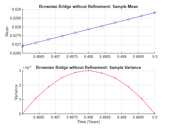
Plot the sample mean and variance of each state variable. The following graph plots the sample statistics of the first state variable only, but similar results hold for any state variable.

subplot(2,1,1);
hold on;
grid on;
plot([T(n) T(n + 1)],[X(n,1) X(n + 1,1)],'.-b')
plot(times, average, 'or')
hold off;
title('Brownian Bridge without Refinement: Sample Mean') 
ylabel('Mean')
limits = axis;
axis([T(n) T(n + 1) limits(3:4)]);

subplot(2,1,2)
hold on;
grid on;
plot(T(n),0,'.-b',T(n + 1),0,'.-b')
plot(times, variance, '.-r')
hold('off');
title('Brownian Bridge without Refinement: Sample Variance')
xlabel('Time (Years)')
ylabel('Variance')
limits = axis;
axis([T(n) T(n + 1) limits(3:4)]);

Figure contains 2 axes objects. Axes object 1 with title Brownian Bridge without Refinement: Sample Mean, ylabel Mean contains 2 objects of type line. One or more of the lines displays its values using only markers Axes object 2 with title Brownian Bridge without Refinement: Sample Variance, xlabel Time (Years), ylabel Variance contains 3 objects of type line.

The Brownian interpolation within the chosen interval, dt, illustrates the following:

  • The conditional mean of each state variable lies on a straight-line segment between the original simulated states at each endpoint.

  • The conditional variance of each state variable is a quadratic function. This function attains its maximum midway between the interval endpoints, and is zero at each endpoint.

  • The maximum variance, although dependent upon the actual model diffusion-rate function G(t,X), is the variance of the sum of NBrowns correlated Gaussian variates scaled by the factor dt/4.

The previous plot highlights interpolation without refinement, in that none of the interpolated states take into account new information as it becomes available. If you had performed interpolation with refinement, new interpolated states would have been inserted into the time series and made available to subsequent interpolations on a trial-by-trial basis. In this case, all random draws for any given interpolation time would be identical. Also, the plot of the sample mean would exhibit greater variability, but would still cluster around the straight-line segment between the original simulated states at each endpoint. The plot of the sample variance, however, would be zero for all interpolation times, exhibiting no variability.

Input Arguments

collapse all

Stochastic differential equation model, specified as an sde, bm, gbm, cev, cir, hwv, heston, sdeddo, sdeld, or sdemrd object.

All MDL parameters are assumed piecewise constant, evaluated from the most recent observation time in Times that precedes a specified interpolation time in T. This is consistent with the Euler approach of Monte Carlo simulation.

Data Types: object

Interpolation times, specified as a NTimes element vector. The length of this vector determines the number of rows in the interpolated output time series XT.

Data Types: double

Sample paths of correlated state variables, specified as a NPeriods-by-NVars-by-NTrials time series array.

For a given trial, each row of this array is the transpose of the state vector Xt at time t. Paths is the initial time series array into which the interpolate function performs the Brownian interpolation.

Data Types: double

Name-Value Arguments

Specify optional pairs of arguments as Name1=Value1,...,NameN=ValueN, where Name is the argument name and Value is the corresponding value. Name-value arguments must appear after other arguments, but the order of the pairs does not matter.

Before R2021a, use commas to separate each name and value, and enclose Name in quotes.

Example: [XT,T] = interpolate(MDL,T,Paths,'Times',t)

Observation times associated with the time series input Paths, specified as the comma-separated pair consisting of 'Times' and a column vector.

Data Types: double

Flag that indicates whether interpolate uses the interpolation times you request (see T) to refine the interpolation as new information becomes available, specified as the comma-separated pair consisting of 'Refine' and a logical with a value of True or False.

Data Types: logical

Sequence of background processes or state vector adjustments, specified as the comma-separated pair consisting of 'Processes' and a function or cell array of functions of the form

Xt=P(t,Xt)

The interpolate function runs processing functions at each interpolation time. They must accept the current interpolation time t, and the current state vector Xt, and return a state vector that may be an adjustment to the input state.

If you specify more than one processing function, interpolate invokes the functions in the order in which they appear in the cell array. You can use this argument to specify boundary conditions, prevent negative prices, accumulate statistics, plot graphs, and so on.

Data Types: cell | function

Output Arguments

collapse all

Interpolated state variables, returned as a NTimes-by-NVars-by-NTrials time series array.

For a given trial, each row of this array is the transpose of the interpolated state vector Xt at time t. XT is the interpolated time series formed by interpolating into the input Paths time series array.

Interpolation times associated with the output time series XT, returned as a NTimes-by-1 column vector.

If the input interpolation time vector Times contains no missing observations (NaNs), the output of T is the same time vector as Times, but with the NaNs removed. This reduces the length of T and the number of rows of XT.

Algorithms

This function performs a Brownian interpolation into a user-specified time series array, based on a piecewise-constant Euler sampling approach.

Consider a vector-valued SDE of the form:

dXt=F(t,Xt)dt+G(t,Xt)dWt

where:

  • X is an NVars-by-1 state vector.

  • F is an NVars-by-1 drift-rate vector-valued function.

  • G is an NVars-by-NBrowns diffusion-rate matrix-valued function.

  • W is an NBrowns-by-1 Brownian motion vector.

Given a user-specified time series array associated with this equation, this function performs a Brownian (stochastic) interpolation by sampling from a conditional Gaussian distribution. This sampling technique is sometimes called a Brownian bridge.

Note

Unlike simulation methods, the interpolation function does not support user-specified noise processes.

  • The interpolate function assumes that all model parameters are piecewise-constant, and evaluates them from the most recent observation time in Times that precedes a specified interpolation time in T. This is consistent with the Euler approach of Monte Carlo simulation.

  • When an interpolation time falls outside the interval specified by Times, a Euler simulation extrapolates the time series by using the nearest available observation.

  • The user-defined time series Paths and corresponding observation Times must be fully observed (no missing observations denoted by NaNs).

  • The interpolate function assumes that the user-specified time series array Paths is associated with the sde object. For example, the Times and Paths input pair are the result of an initial course-grained simulation. However, the interpolation ignores the initial conditions of the sde object (StartTime and StartState), allowing the user-specified Times and Paths input series to take precedence.

References

[1] Ait-Sahalia, Y. “Testing Continuous-Time Models of the Spot Interest Rate.” The Review of Financial Studies, Spring 1996, Vol. 9, No. 2, pp. 385–426.

[2] Ait-Sahalia, Y. “Transition Densities for Interest Rate and Other Nonlinear Diffusions.” The Journal of Finance, Vol. 54, No. 4, August 1999.

[3] Glasserman, P. Monte Carlo Methods in Financial Engineering. New York, Springer-Verlag, 2004.

[4] Hull, J. C. Options, Futures, and Other Derivatives, 5th ed. Englewood Cliffs, NJ: Prentice Hall, 2002.

[5] Johnson, N. L., S. Kotz, and N. Balakrishnan. Continuous Univariate Distributions. Vol. 2, 2nd ed. New York, John Wiley & Sons, 1995.

[6] Shreve, S. E. Stochastic Calculus for Finance II: Continuous-Time Models. New York: Springer-Verlag, 2004.

Version History

Introduced in R2008a