Bond Portfolio CVaR Optimization Using Diebold-Li Model

This example shows how to perform bond portfolio optimization by using the Diebold-Li dynamic factor model of the yield curve to simulate and compute bond returns.

For observation date $\mathit{t}$ and time to maturity $\tau$, the Diebold-Li model of the yield is given by

${\mathit{y}}_{\mathit{t}}\left(\tau \right)={\mathit{L}}_{\mathit{t}}+{\mathit{S}}_{\mathit{t}}\left(\frac{1-{\mathit{e}}^{-\lambda \tau }}{\lambda \tau }\right)+{\mathit{C}}_{\mathit{t}}\left(\frac{1-{\mathit{e}}^{-\lambda \tau }}{\lambda \tau }-{\mathit{e}}^{-\lambda \tau }\right)$,

where:

• ${\mathit{L}}_{\mathit{t}}$ is the long-term factor (level).

• ${\mathit{S}}_{\mathit{t}}$ is the short-term factor (slope).

• ${\mathit{C}}_{\mathit{t}}$ is the medium-term factor (curvature).

• $\lambda$ determines the maturity at which the loading curve is maximized and goversn the exponential decay rate of the model.

State-Space Formulation of Diebold-Li Model

In this example, you use the model from the Apply State-Space Methodology to Analyze Diebold-Li Yield Curve Model (Econometrics Toolbox) example to calculate the monthly returns. The associated ssm (Econometrics Toolbox) model is described in Load Yield Curve Data and ssm Model.

The level, slope, and curvature factors of the Diebold-Li model follow the state transition equation given by

$$\left[\begin{array}{c}{\mathit{L}}_{\mathit{t}}-{\mu }_{\mathit{L}}\\ {\mathit{S}}_{\mathit{t}}-{\mu }_{\mathit{S}}\\ {\mathit{C}}_{\mathit{t}}-{\mu }_{\mathit{C}}\end{array}\right]=\left[\begin{array}{ccc}{\mathit{a}}_{11}& {\mathit{a}}_{12}& {\mathit{a}}_{13}\\ {\mathit{a}}_{21}& {\mathit{a}}_{22}& {\mathit{a}}_{23}\\ {\mathit{a}}_{31}& {\mathit{a}}_{32}& {\mathit{a}}_{33}\end{array}\right]\left[\begin{array}{c}{\mathit{L}}_{\mathit{t}-1}-{\mu }_{\mathit{L}}\\ {\mathit{S}}_{\mathit{t}-1}-{\mu }_{\mathit{S}}\\ {\mathit{C}}_{\mathit{t}-1}-{\mu }_{\mathit{C}}\end{array}\right]+\left[\begin{array}{c}{\eta }_{\mathrm{Lt}}\\ {\eta }_{\mathrm{St}}\\ {\eta }_{\mathrm{Ct}}\end{array}\right]$$

where $\mu$ is the vector of means for each factor, and the corresponding observation equation is

$$\left[\begin{array}{c}{\mathit{y}}_{{\tau }_1\mathit{t}}\\ {\mathit{y}}_{{\tau }_2\mathit{t}}\\ ⋮\\ {\mathit{y}}_{{\tau }_{\mathit{N}}\mathit{t}}\end{array}\right]=\left[\begin{array}{ccc}1& \frac{1-{\mathit{e}}^{-\lambda {\tau }_1}}{\lambda {\tau }_1}& \frac{1-{\mathit{e}}^{-\lambda {\tau }_1}}{\lambda {\tau }_1}-{\mathit{e}}^{-\lambda {\tau }_1}\\ 1& \frac{1-{\mathit{e}}^{-\lambda {\tau }_2}}{\lambda {\tau }_2}& \frac{1-{\mathit{e}}^{-\lambda {\tau }_2}}{\lambda {\tau }_2}-{\mathit{e}}^{-\lambda {\tau }_2}\\ ⋮& ⋮& ⋮\\ 1& \frac{1-{\mathit{e}}^{-\lambda {\tau }_{\mathit{N}}}}{\lambda {\tau }_{\mathit{N}}}& \frac{1-{\mathit{e}}^{-\lambda {\tau }_{\mathit{N}}}}{\lambda {\tau }_{\mathit{N}}}-{\mathit{e}}^{-\lambda {\tau }_{\mathit{N}}}\end{array}\right]\left[\begin{array}{c}{\mathit{L}}_{\mathit{t}}\\ {\mathit{S}}_{\mathit{t}}\\ {\mathit{C}}_{\mathit{t}}\end{array}\right]+\left[\begin{array}{c}{\epsilon }_{{\tau }_1\mathit{t}}\\ {\epsilon }_{{\tau }_2\mathit{t}}\\ ⋮\\ {\epsilon }_{{\tau }_{\mathit{N}}\mathit{t}}\end{array}\right]$$

You can represent these two sets of equations in the following vector representation

$$\begin{array}{l}\left({\mathit{f}}_{\mathit{t}}-\mu \right)=\mathit{A}\left({\mathit{f}}_{\mathit{t}-1}-\mu \right)+{\eta }_{\mathit{t}}\\ {\mathit{y}}_{\mathit{t}}=\Lambda {\mathit{f}}_{\mathit{t}}+{\epsilon }_{\mathit{t}}\end{array}$$

If you define the latent states ${\mathit{x}}_{\mathit{t}}$ as the mean-adjusted factors

$${\mathit{x}}_{\mathit{t}}={\mathit{f}}_{\mathit{t}}-\mu$$

and define the deflated yields $\stackrel{\sim }{{\mathit{y}}_{\mathit{t}}}$ as

$$\stackrel{\sim }{{\mathit{y}}_{\mathit{t}}}={\mathit{y}}_{\mathit{t}}-\Lambda \mu$$

then you can substitute ${\mathit{x}}_{\mathit{t}}$ and $\stackrel{\sim }{{\mathit{y}}_{\mathit{t}}}$ into the preceding equations to obtain the following Diebold-Li state-space system:

$$\begin{array}{l}{\mathit{x}}_{\mathit{t}}=\mathit{A}{\mathit{x}}_{\mathit{t}-1}+{\eta }_{\mathit{t}}\\ \stackrel{\sim }{{\mathit{y}}_{\mathit{t}}}=\Lambda {\mathit{x}}_{\mathit{t}}+{\epsilon }_{\mathit{t}}\end{array}$$

Load Yield Curve Data and ssm Model

The yield data consists of 29 years of monthly, unsmoothed Fama-Bliss US Treasury zero-coupon yield measurements. The time series in the data represents maturities of 3, 6, 9, 12, 15, 18, 21, 24, 30, 36, 48, 60, 72, 84, 96, 108, and 120 months. The data expresses the yields in percents and records them at the end of each month, beginning January 1972 and ending December 2000, for a total of 348 monthly curves of 17 maturities each.

Load the Diebold-Li data set and extract the yield series.

load("Data_DieboldLi.mat")
yieldsMaturity = maturities';
yields = DataTimeTable{:,1:17};

Load the Diebold-Li yield curve model.

load("EstimatedDieboldLiSSM.mat")

Simulate Bond Returns

To simulate bond returns for the following investment period ($\mathit{t}+1$), follow these steps:

1. Price bonds at time period $\mathit{t}$ by using the zero-coupon bond yield curve, also known as the zero curve. Since some bonds have cash flows whose time to maturity do not match one of the tenors in the zero curve, you must use interpolation.

2. Simulate the $\mathit{t}+1$ zero curve by using the period $\mathit{t}$ factor estimates and their covariance matrix.

3. Price bonds at time period $\mathit{t}+1$ by using the simulated zero curves.

4. Compute simulated returns by using the following formula for each bond $\mathit{i}$:

$$\frac{\left({\mathit{P}}_{\mathit{i}\left(\mathit{t}+1\right)}-{\mathit{P}}_{\mathrm{it}}\right)}{{\mathit{P}}_{\mathrm{it}}}$$

Start by loading the bonds information.

load('BondsCouponsAndMaturities')
couponRate = bondsTable.CouponRate;
bondsMaturity = bondsTable.Maturity;

Define the purchase date as the date at the end of the time horizon.

settle = DataTimeTable.Time(end);

Generate bonds cash flow amounts and time mapping.

[CFAmounts,CFDates] = cfamounts(couponRate,settle,bondsMaturity);
[allCF,allDates] = cfport(CFAmounts,CFDates);

Interpolate existing yields to obtain yields at cash flow times.

% Compute yields times
yieldsDates = settle + calmonths(yieldsMaturity);
yieldsTimes = yearfrac(settle,yieldsDates);
yieldsT = yields(end,:)/100;

% Interpolate to obtain yields at cash flow times
CFTimes = yearfrac(settle,allDates);
CFYields = interp1(yieldsTimes,yieldsT,CFTimes,[],"extrap");

Compute prices assuming continuous compounding.

% Compute prices from cash flow yields
DF = exp(-CFYields.*CFTimes);
bondsPrices = (allCF*DF)';

To simulate the yield curve at time period $\mathit{t}+1$, first obtain the period $\mathit{t}$ state mean and covariance matrix by using smooth (Econometrics Toolbox) with the deflated yields $\stackrel{\sim }{{\mathit{y}}_{\mathit{t}}}$. The final element of the output structure corresponds to the mean and covariance of the smoothed estimate at time period $\mathit{t}$.

% Deflate the yields
intercept = (EstMdlSSM.C*mu')';
deflatedYields = yields - intercept;

% Obtain period t state mean and covariance
[~,~,output] = smooth(EstMdlSSM,deflatedYields);
MeanT = output(end).SmoothedStates;
CovT = output(end).SmoothedStatesCov;
CovT = (CovT + CovT')/2; % Ensures covariance is symmetric

Then, set the states initial mean and covariance of EstMdlSSM to the state mean and covariance at time period $\mathit{t}$.

% Set the initial state mean and covariance to the estimates at T
EstMdlSSM.Mean0 = MeanT;
EstMdlSSM.Cov0 = CovT;

Simulate 100,000 one-month-ahead deflated yields from the state-space model and then inflate the yields.

% Simulate 100,000 yields
rng('default')
simDeflatedYields = simulate(EstMdlSSM,1,NumPaths=1e5);
simDeflatedYields = squeeze(simDeflatedYields(:,:,:));
simDeflatedYields = simDeflatedYields';

% Inflate yields
simYields = (simDeflatedYields + intercept)/100;

Use simulated yields to compute simulation of prices at time $\mathit{t}+1$.

% Set new settle date
simSettle = settle + calmonths(1);

% Interpolate simulated yields at cash flow times
simCFTimes = yearfrac(simSettle,allDates);
simCFYields = interp1(yieldsTimes,simYields',simCFTimes',[],"extrap")';

% Compute prices from cash flow yields
simDF = exp(-simCFYields.*simCFTimes');
simBondsPrices = (allCF*simDF')';

% Compute simulated returns
simMonthlyReturns = (simBondsPrices - bondsPrices)./bondsPrices;

The resulting returns simulation allows you to analyze the distribution of the one-month-ahead returns of the bonds. You can plot the distribution of the one-month-ahead distribution of the bonds with 3-month, 10-year, and 20-year maturities.

figure
t = tiledlayout(3,1);
title(t,'PDF of One-Month-Ahead Returns')
ylabel(t,'Returns')
bins = -0.1:0.001:0.1;

% 3-month maturity bond
nexttile
histogram(simMonthlyReturns(:,3),bins,'Normalization','pdf')
xlabel('3-Month Maturity Bond')

% 24-month maturity
nexttile
histogram(simMonthlyReturns(:,68),'Normalization','pdf')
xlabel('10-Year Maturity Bond')

% 120-month maturity
nexttile
histogram(simMonthlyReturns(:,90),'Normalization','pdf')
xlabel('20-Year Maturity Bond')

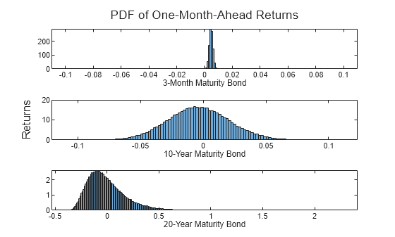
As the maturity increases, the variance of the returns increases and the distribution gets positively skewed.

Solve CVaR Bond Portfolio Optimization

Now use the simulated returns (simMonthlyReturns) to solve conditional value-at-risk (CVaR) optimization problems of fixed-income portfolios.

To solve the CVaR problem, use the PortfolioCVaR object. The optimal portfolio must invest in at least 10 types of bonds and no more than 30. At least 5% of the portfolio value must be invested in any chosen bond. This example also requires that you invest the entire capital in the portfolio.

% 95% CVaR Portfolio
p = PortfolioCVaR(Scenarios=simMonthlyReturns,ProbabilityLevel=0.95);

% Semi-continuous bounds
p = setBounds(p,0.05,0.5,BoundType="conditional");

% Cardinality constraint
p = setMinMaxNumAssets(p,10,30);

% Fully-invested portfolio
p = setBudget(p,1,1);

Use setInequality to add a constraint to the portfolio duration to match a given benchmark portfolio duration.

% Duration constraint
targetDuration = 10;
durationTol = 1;
bondsDuration = bnddurp(bondsPrices,couponRate,settle,bondsMaturity);
p = setInequality(p,[bondsDuration';-bondsDuration'], ...
    [targetDuration+durationTol;durationTol-targetDuration]);

Use setCosts to account for the impact of transaction costs when computing the return of the portfolio.

% Transaction costs
cost = 3e-4; % 3 bps
w0 = zeros(p.NumAssets,1);
w0([1 2 3 4 16 18 19 20]) = 0.05;
w0(110) = 0.1;
w0(112) = 0.5;
p = setCosts(p,cost,cost,w0);

Use estimateFrontier to compute the efficient frontier and then use plotFrontier to plot the efficient frontier of the portfolio problem.

% Plot efficient frontier
figure
pwgt = estimateFrontier(p);
plotFrontier(p,pwgt)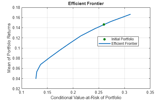

The plot shows that the minimum risk portfolio achieves a CVaR of 12.91% with an associated return of 4.10%, while the maximum return portfolio has a CVaR of 30.93% and a return of 15.94%.

% Table of efficient portfolio non-zero weights
idxNonZero = sum(pwgt >= 1e-4,2) >= 1;
nonZeroWeightsTable = array2table(pwgt(idxNonZero,:), ...
    RowNames=string(bondsMaturity(idxNonZero)), ...
    VariableNames="Portfolio"+string(1:10))

nonZeroWeightsTable=28×10 table
                  Portfolio1    Portfolio2    Portfolio3    Portfolio4    Portfolio5     Portfolio6    Portfolio7    Portfolio8    Portfolio9    Portfolio10
                  __________    __________    __________    __________    ___________    __________    __________    __________    __________    ___________

    2001-02-15          0             0             0         0.062484       0.050084           0       0.057716      0.088604      0.063725      0.076125  
    2001-02-28          0             0             0                0     1.3553e-20     0.05025           0.05          0.05          0.05          0.05  
    2001-03-31          0             0             0                0           0.05           0           0.05          0.05          0.05          0.05  
    2001-04-30          0             0             0       8.6736e-18           0.05           0           0.05          0.05          0.05          0.05  
    2001-05-15          0             0             0       3.4694e-18    -1.7618e-19           0              0          0.05          0.05          0.05  
    2001-05-31          0             0             0                0     1.3553e-20           0              0          0.05          0.05             0  
    2001-06-30          0             0             0                0              0           0              0             0          0.05             0  
    2002-01-31          0             0             0                0              0        0.05              0             0             0             0  
    2002-02-28          0             0             0                0              0        0.05           0.05          0.05             0             0  
    2002-03-31          0             0             0                0              0        0.05           0.05             0             0             0  
    2002-04-30          0             0             0                0    -8.6736e-19        0.05              0             0             0             0  
    2007-11-15          0             0             0             0.05     1.5613e-17           0              0             0             0             0  
    2008-02-15          0             0          0.05                0              0           0              0             0             0             0  
    2008-05-15          0             0          0.05             0.05              0           0              0             0             0             0  
    2008-11-15          0          0.05          0.05             0.05           0.05           0              0             0             0             0  
    2009-05-15       0.05          0.05          0.05             0.05           0.05        0.05              0             0             0             0  
      ⋮

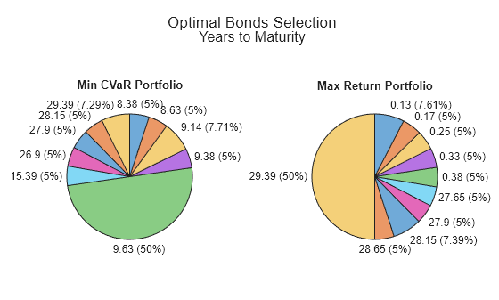
The table shows how the least risky portfolios invest more on bonds with a maturity of approximately 9 years and, as the return levels increase, the investment concetrates on bonds with longer maturities.

% Compare weights of min risk and max return portfolios
labels = yearfrac(settle,bondsMaturity);
labels = round(labels,2);

% Plot pie charts
figure
t = tiledlayout(1,2);
title(t,'Optimal Bonds Selection','Years to Maturity')

% Min CVaR portfolio
nexttile
idxMinCVaR = pwgt(:,1) >= 1e-4;
piechart(pwgt(idxMinCVaR,1),labels(idxMinCVaR))
title('Min CVaR Portfolio')

% Max return portfolio
nexttile
idxMaxRet = pwgt(:,end) >= 1e-4;
piechart(pwgt(idxMaxRet,end),labels(idxMaxRet))
title('Max Return Portfolio')