estimate

Fit threshold-switching dynamic regression model to data

Since R2021b

Syntax

EstMdl = estimate(Mdl,tt0,Y)

EstMdl = estimate(Mdl,tt0,Y,Name,Value)

[EstMdl,logL] = estimate(___)

[EstMdl,logL] = estimate(ax,___)

[EstMdl,logL,h] = estimate(ax,___)

Description

EstMdl = estimate(Mdl,tt0,Y) estimates parameters of the threshold-switching dynamic regression model Mdl. estimate fits the model to the response data Y, and initializes the estimation procedure by treating the parameter values of the fully specified threshold transitions tt0 as initial values. estimate implements a version of the conditional least-squares algorithm described in [4].

EstMdl = estimate(Mdl,tt0,Y,Name,Value) uses additional options specified by one or more name-value arguments. For example, estimate(Mdl,tt0,Y,IterationPlot=true) displays a plot of the loglikelihood versus the iteration step, after the algorithm terminates.

[EstMdl,logL] = estimate(___) also returns the estimated loglikelihood logL when the algorithm terminates, using any of the input argument combinations in the previous syntaxes.

[EstMdl,logL] = estimate(ax,___) plots iterations on the axes specified by ax instead of the current axes (gca). The option ax can precede any of the input argument combinations in the previous syntaxes.

[EstMdl,logL,h] = estimate(ax,___) also returns the plot handle h. Use h to modify properties of the plot after you create it.

Examples

Fit SETAR Model to Simulated Data

Assess estimation accuracy using simulated data from a known data-generating process (DGP). This example uses arbitrary parameter values.

Create Model for DGP

Create a discrete threshold transition at mid-level 1.

ttDGP = threshold(1)

ttDGP = 
  threshold with properties:

          Type: 'discrete'
        Levels: 1
         Rates: []
    StateNames: ["1"    "2"]
     NumStates: 2

ttDGP is a threshold object representing the state-switching mechanism of the DGP.

Create the following fully specified self-exciting TAR (SETAR) model for the DGP.

• State 1: ${\mathit{y}}_{\mathit{t}}={\epsilon }_{\mathit{t}}$.

• State 2: ${\mathit{y}}_{\mathit{t}}=2+{\epsilon }_{\mathit{t}}$.

• ${\epsilon }_{\mathit{t}}\sim {\rm N}\left(0,1\right)$.

Specify the submodels by using arima.

mdl1DGP = arima(Constant=0);
mdl2DGP = arima(Constant=2);
mdlDGP = [mdl1DGP mdl2DGP];

Because the innovations distribution is invariant across states, the tsVAR software ignores the value of the submodel innovations variance (Variance property).

Create a threshold-switching model for the DGP. Specify the model-wide innovations variance.

MdlDGP = tsVAR(ttDGP,mdlDGP,Covariance=1);

MdlDGP is a tsVAR object representing the DGP.

Simulate Response Paths from DGP

Generate a random response path of length 100 from the DGP. By default, simulate assumes a SETAR model with delay $\mathit{d}=1$. In other words, the threshold variable is ${\mathit{y}}_{\mathit{t}-1}$.

rng(1) % For reproducibiliy
y = simulate(MdlDGP,100);

y is a 100-by-1 vector of representing the simulated response path.

Create Model for Estimation

Create a partially specified threshold-switching model that has the same structure as the data-generating process, but specify the transition mid-level, submodel coefficients, and model-wide constant as unknown for estimation.

tt = threshold(NaN);
mdl1 = arima('Constant',NaN);
mdl2 = arima('Constant',NaN);
Mdl = tsVAR(tt,[mdl1,mdl2],'Covariance',NaN);

Mdl is a partially specified tsVAR object representing a template for estimation. NaN-valued elements of the Switch and Submodels properties indicate estimable parameters.

Mdl is agnostic of the threshold variable; tsVAR object functions enable you to specify threshold variable characteristics or data.

Create Threshold Transitions Containing Initial Values

The estimation procedure requires initial values for all estimable threshold transition parameters.

Fully specify a threshold transition that has the same structure as tt, but set the mid-level to 0.

tt0 = threshold(0);

tt0 is a fully specified threshold object.

Estimate Model

Fit the model to the simulated path. By default, the model is self-exciting and the delay of the threshold variable is $\mathit{d}=1$.

EstMdl = estimate(Mdl,tt0,y)

EstMdl = 
  tsVAR with properties:

         Switch: [1×1 threshold]
      Submodels: [2×1 varm]
      NumStates: 2
      NumSeries: 1
     StateNames: ["1"    "2"]
    SeriesNames: "1"
     Covariance: 1.0225

EstMdl is a fully specified tsVAR object representing the estimated SETAR model.

Display an estimation summary of the submodels.

summarize(EstMdl)

Description
1-Dimensional tsVAR Model with 2 Submodels

Switch
Transition Type: discrete
Estimated Levels: 1.128

Fit
Effective Sample Size: 99 
Number of Estimated Parameters: 2 
Number of Constrained Parameters: 0 
LogLikelihood: -141.574 
AIC: 287.149 
BIC: 292.339 

Submodels
                           Estimate    StandardError    TStatistic      PValue  
                           ________    _____________    __________    __________

    State 1 Constant(1)    -0.12774       0.13241        -0.96474        0.33467
    State 2 Constant(1)      2.1774       0.16829          12.939     2.7264e-38

The estimates are close to their true values.

Plot the estimated switching mechanism with the threshold data, which is the response data.

figure
ttplot(EstMdl.Switch,'Data',y)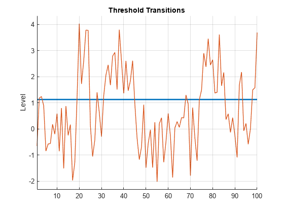

Tune Delay Parameter for SETAR Estimation

estimate does not fit the delay parameter $\mathit{d}$ to the data; you must specify its value when you call estimate. This example shows how to tune $\mathit{d}$.

Create the following fully specified SETAR model for the DGP.

• State 1: ${\mathit{y}}_{\mathit{t}}={\epsilon }_{1,\mathit{t}}$, where ${\epsilon }_{1,\mathit{t}}\sim {\rm N}\left(0,1\right)$.

• State 2: ${\mathit{y}}_{\mathit{t}}=2+{\epsilon }_{2,\mathit{t}}$, where ${\epsilon }_{2,\mathit{t}}\sim {\rm N}\left(0,2\right)$.

• The system is in state 1 when ${\mathit{y}}_{\mathit{t}-4}<0$, and it is in state 2 otherwise.

ttDGP = threshold(0);
mdl1DGP = arima(Constant=0,Variance=1);
mdl2DGP = arima(Constant=2,Variance=2);
mdlDGP = [mdl1DGP; mdl2DGP];
MdlDGP = tsVAR(ttDGP,mdlDGP);

Generate a random response path of length 200 from the DGP. Specify that the threshold variable delay is 4.

rng(1) % For reproducibiliy
y = simulate(MdlDGP,200,Delay=4);

plot(y)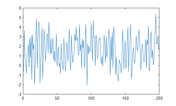

Create a partially specified threshold-switching model that has the same structure as the data-generating process, but specify the transition mid-level, submodel coefficients, and state-specific variances as unknown for estimation.

tt = threshold(NaN);
mdl = arima(0,0,0);
Mdl = tsVAR(tt,[mdl; mdl]);

Fully specify a threshold transition that has the same structure as tt, but set the mid-level to 0.5.

tt0 = threshold(0.5);

Tune $\mathit{d}$ by choosing a set of plausible values for it, and by fitting the SETAR model to the simulated data for each value in the set. Choose the model that maximizes the loglikelihood.

d = 1:8;
nd = numel(d);
logL = zeros(nd,1);     % Preallocate for loglikelihoods
EstMdl = cell(nd,1);    % Preallocate for estimated models

for j = 1:nd
    [EstMdl{j},logL(j)] = estimate(Mdl,tt0,y,Delay=d(j));
end

Extract the model that maximizes the loglikelihood.

[~,optDelay] = max(logL)

optDelay = 
4

OptEstMdl = EstMdl{optDelay};

The optimal delay is 4, which matches the delay of the DGP.

Display an estimation summary of the optimal model, and display its estimated switching mechanism.

summarize(OptEstMdl)

Description
1-Dimensional tsVAR Model with 2 Submodels

Switch
Transition Type: discrete
Estimated Levels: -0.063

Fit
Effective Sample Size: 196 
Number of Estimated Parameters: 2 
Number of Constrained Parameters: 0 
LogLikelihood: -336.184 
AIC: 676.367 
BIC: 682.923 

Submodels
                           Estimate    StandardError    TStatistic      PValue  
                           ________    _____________    __________    __________

    State 1 Constant(1)    -0.33535       0.24271        -1.3817         0.16707
    State 2 Constant(1)      2.0073       0.10647         18.853      2.7794e-79

The estimates are close to the parameters of the DGP.

Plot Loglikelihood Evolution During Multivariate SETAR Estimation

Create the following fully specified SETAR model for the DGP.

• State 1: $$\left[\begin{array}{c}{y}_{1,t}\\ y_{2,t}\end{array}\right]=\left[\begin{array}{c}-1\\ -4\end{array}\right]+\left[\begin{array}{cc}-0.5& 0.1\\ 0.2& -0.75\end{array}\right]\left[\begin{array}{c}{y}_{1,t-1}\\ y_{2,t-1}\end{array}\right]+\left[\begin{array}{c}{\epsilon }_{1,t}\\ {\epsilon }_{2,t}\end{array}\right]$$.

• State 2: $$\left[\begin{array}{c}{y}_{1,t}\\ y_{2,t}\end{array}\right]=\left[\begin{array}{c}1\\ 4\end{array}\right]+\left[\begin{array}{c}{\epsilon }_{1,t}\\ {\epsilon }_{2,t}\end{array}\right]$$.

• State 3:$$\left[\begin{array}{c}{y}_{1,t}\\ y_{2,t}\end{array}\right]=\left[\begin{array}{c}1\\ 4\end{array}\right]+\left[\begin{array}{cc}0.5& 0.1\\ 0.2& 0.75\end{array}\right]\left[\begin{array}{c}{y}_{1,t-1}\\ y_{2,t-1}\end{array}\right]+\left[\begin{array}{c}{\epsilon }_{1,t}\\ {\epsilon }_{2,t}\end{array}\right]$$.

• $$\left[\begin{array}{c}{\epsilon }_{1,t}\\ {\epsilon }_{2,t}\end{array}\right]\sim N_2(\left[\begin{array}{c}0\\ 0\end{array}\right],\left[\begin{array}{cc}2& -1\\ -1& 1\end{array}\right])$$.

• The system is in state 1 when ${\mathit{y}}_{2,\mathit{t}-4}<-3$, the system is in state 2 when $-3\le {\mathit{y}}_{2,\mathit{t}-4}<$3, and the system is in state 3 otherwise.

t = [-3 3];
ttDGP = threshold(t);

constant1 = [-1; -4];
constant2 = [1; 4];
constant3 = [1; 4];
AR1 = [-0.5 0.1; 0.2 -0.75];
AR3 = [0.5 0.1; 0.2 0.75];
Sigma = [2 -1; -1 1];

mdl1DGP = varm(Constant=constant1,AR={AR1});
mdl2DGP = varm(Constant=constant2);
mdl3DGP = varm(Constant=constant3,AR={AR3});

mdlDGP = [mdl1DGP; mdl2DGP; mdl3DGP];
MdlDGP = tsVAR(ttDGP,mdlDGP,Covariance=Sigma);

Generate a random response path of length 500 from the DGP. Specify that second response variable with a delay of 4 as the threshold variable.

rng(10) % For reproducibiliy
y = simulate(MdlDGP,500,Index=2,Delay=4);

Create a partially specified threshold-switching model that has the same structure as the DGP, but specify the transition mid-level, submodel coefficients, and model-wide covariance as unknown for estimation.

tt = threshold([NaN; NaN]);
mdlar = varm(2,1);
mdlc = varm(2,0);
Mdl = tsVAR(tt,[mdlar; mdlc; mdlar],Covariance=nan(2));

Fully specify a threshold transition that has the same structure as tt, but set the mid-levels to -1 and 1.

t0 = [-1 1];
tt0 = threshold(t0);

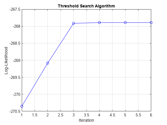
Fit the threshold-switching model to the simulated series. Specify the threshold variable ${\mathit{y}}_{2,\mathit{t}-4}$. Plot the loglikelihood after each iteration of the threshold search algorithm.

EstMdl = estimate(Mdl,tt0,y,IterationPlot=true,Index=2,Delay=4);

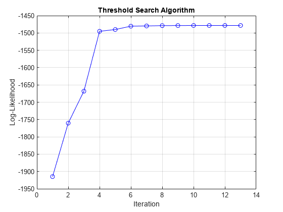
The plot displays the evolution of the loglikelihood as the estimation procedure searches for optimal levels. The procedure terminates when one of the stopping criteria is satisfied.

Display an estimation summary of the model.

summarize(EstMdl)

Description
2-Dimensional tsVAR Model with 3 Submodels

Switch
Transition Type: discrete
Estimated Levels: -2.877  2.991

Fit
Effective Sample Size: 496 
Number of Estimated Parameters: 14 
Number of Constrained Parameters: 0 
LogLikelihood: -1478.416 
AIC: 2984.831 
BIC: 3043.723 

Submodels
                           Estimate    StandardError    TStatistic      PValue   
                           ________    _____________    __________    ___________

    State 1 Constant(1)     -1.0369       0.13859        -7.4821        7.312e-14
    State 1 Constant(2)     -4.0179       0.09959        -40.345                0
    State 1 AR{1}(1,1)     -0.43289      0.063204        -6.8491       7.4332e-12
    State 1 AR{1}(2,1)      0.20344      0.045419         4.4791       7.4957e-06
    State 1 AR{1}(1,2)     0.076123      0.024477         3.1099        0.0018714
    State 1 AR{1}(2,2)     -0.75607       0.01759        -42.983                0
    State 2 Constant(1)      1.0545       0.14882         7.0858        1.382e-12
    State 2 Constant(2)      4.1131       0.10694          38.46      1.9763e-323
    State 3 Constant(1)      1.0621      0.095701         11.098       1.2802e-28
    State 3 Constant(2)      3.8707      0.068772         56.284                0
    State 3 AR{1}(1,1)      0.47396      0.058016         8.1694       3.0997e-16
    State 3 AR{1}(2,1)      0.23013      0.041691         5.5199       3.3927e-08
    State 3 AR{1}(1,2)      0.10561      0.018233         5.7924       6.9371e-09
    State 3 AR{1}(2,2)       0.7568      0.013102         57.761                0

Specify Presample Data for STAR Model Estimation

Consider a smooth threshold-switching (STAR) model for the real US GDP growth rate, where each submodel is AR(4) and the threshold variable is the unemployment growth rate.

Create a partially specified threshold transition for the unemployment growth rate. Specify the normal cdf transition function, and an unknown, estimable mid-level and rate. Label the states "Contraction" and "Expansion".

tt = threshold(NaN,Type="normal",Rates=NaN, ...
    StateNames=["Contraction" "Expansion"]);

tt is a partially specified threshold object, and it is agnostic of the variable and data it represents.

Create a threshold-switching model for the real US GDP growth rate. Label the series "rRGDP".

mdl = arima(4,0,0);
submdls = [mdl; mdl];
Mdl = tsVAR(tt,submdls,SeriesNames="rRGDP");

Load the quarterly US macroeconomic data set Data_USEconModel.mat. Compute the real GDP percent growth and unemployment growth.

load Data_USEconModel

DataTimeTable = rmmissing(DataTimeTable,DataVariables=["GDP" "GDPDEF" "UNRATE"]);
RGDP = DataTimeTable.GDP./DataTimeTable.GDPDEF;
rRGDP = price2ret(RGDP)*100;            % Response data
gUNRATE = diff(DataTimeTable.UNRATE);   % Exogenous thresold data
dates = DataTimeTable.Time(2:end);

Suppose the estimation period includes growth rates from the first quarter of 1950. Identify the estimation period in the date base.

startEst = datetime(1950,1,1);
idxEst = dates >= startEst;

To initialize the estimation procedure, fully specify a threshold transition that has the same structure as tt, but set the mid-level to -0.5 with a rate of 100.

tt0 = threshold(-0.5,Type=tt.Type,Rates=100,StateNames=tt.StateNames);

Fit the STAR model to the estimation period of the US GDP growth rate series. Specify the following parameters:

• Set Y0 to the responses before the estimation period to initialize the AR submodel components.

• Set Type to "exogenous" to characterize the threshold variable.

• Set Z to the threshold variable data gUNRATE in the estimation period.

• Set MaxRate to 150 to expand the search for the optimal transition function rate.

• Plot the evolution of the loglikelihood.

EstMdl = estimate(Mdl,tt0,rRGDP(idxEst),Y0=rRGDP(~idxEst), ...
    Z=gUNRATE(idxEst),Type="exogenous",MaxRate=150,IterationPlot=true);

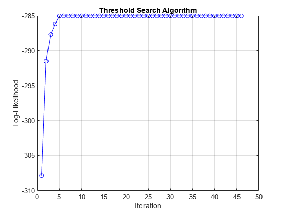
Display an estimation summary and plot the estimated switching mechanism with the threshold data.

summarize(EstMdl)

Description
1-Dimensional tsVAR Model with 2 Submodels

Switch
Transition Type: normal
Estimated Levels: 0.208
Estimated Rates: 75.566

Fit
Effective Sample Size: 237 
Number of Estimated Parameters: 10 
Number of Constrained Parameters: 0 
LogLikelihood: -285.022 
AIC: 590.043 
BIC: 624.724 

Submodels
                           Estimate     StandardError    TStatistic      PValue  
                           _________    _____________    __________    __________

    State 1 Constant(1)       1.0473       0.11549           9.068     1.2125e-19
    State 1 AR{1}(1,1)       0.15792      0.068783          2.2959       0.021679
    State 1 AR{2}(1,1)      0.059888      0.066409          0.9018        0.36716
    State 1 AR{3}(1,1)      -0.10455      0.070384         -1.4854        0.13744
    State 1 AR{4}(1,1)     -0.098037      0.063249           -1.55        0.12114
    State 2 Constant(1)     -0.12491       0.15383        -0.81197        0.41681
    State 2 AR{1}(1,1)       0.15366       0.13993          1.0981        0.27215
    State 2 AR{2}(1,1)     -0.027925       0.16754        -0.16667        0.86763
    State 2 AR{3}(1,1)      -0.24366       0.12778         -1.9068       0.056543
    State 2 AR{4}(1,1)     -0.075389       0.14024        -0.53759        0.59086

figure
ttplot(EstMdl.Switch,Data=gUNRATE(idxEst))
dEst = dates(idxEst);
xticklabels(string(dEst(xticks)))

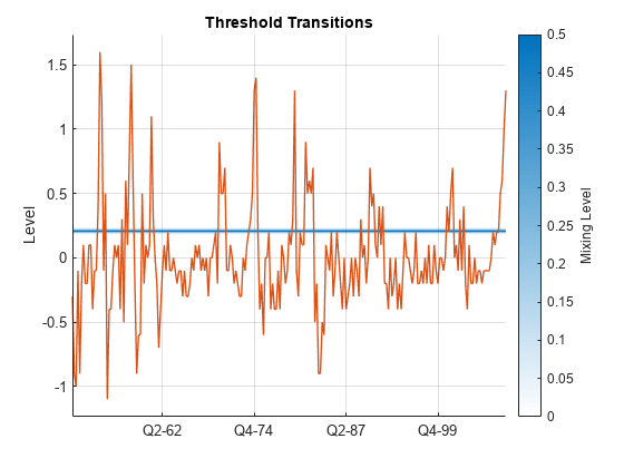
The large rate suggests little mixing occurs between the models of each regime. When the quarterly unempoyment growth is less than 0.206%, the dominant model for the US GDP growth rate is in EstMdl.Submodels(1). Otherwise, the dominant submodel is in EstMdl.Submodels(2).

Many of the coefficients are insignificant, which can suggest a search for a simpler model.

Perform Constrained Estimation

This example shows how to specify equality constraints on estimable submodel coefficients and threshold parameters.

Consider the model for the real US GDP growth rate in Specify Presample Data for STAR Model Estimation. Assume the submodels are AR(4), but they include only the model constant (time trend in differenced series) and fourth lag. Also, suppose the transition function rate 3 for the unemployment growth series.

Create the partially specified threshold transition for the unemployment growth rate. Specify the known transition rate.

rConstraint = 3;
tt = threshold(NaN,Type="normal",Rates=rConstraint, ...
    StateNames=["Contraction" "Expansion"]);

Create a threshold-switching model for the real US GDP growth rate. Explicitly specify the AR lags to include in the submodels by using the ARLags option.

mdl = arima(ARLags=4);
submdls = [mdl; mdl];
Mdl = tsVAR(tt,submdls,SeriesNames="rRGDP");

Load the quarterly US macroeconomic data set Data_USEconModel.mat. Compute the real GDP percent growth and unemployment growth.

load Data_USEconModel

DataTimeTable = rmmissing(DataTimeTable,DataVariables=["GDP" "GDPDEF" "UNRATE"]);
RGDP = DataTimeTable.GDP./DataTimeTable.GDPDEF;
rRGDP = price2ret(RGDP)*100;        % Response data
gUNRATE = diff(DataTimeTable.UNRATE);   % Exogenous thresold data
dates = DataTimeTable.Time(2:end);

Suppose the estimation period includes growth rates from the first quarter of 1950. Identify the estimation period in the date base.

startEst = datetime(1950,1,1);
idxEst = dates >= startEst;

Fully specify a threshold transition that has the same structure as tt, including the equality constraint on the transition function rate. Set the initial mid-level to 0.

tt0 = threshold(0,Type=tt.Type,Rates=rConstraint,StateNames=tt.StateNames);

Fit the STAR model to the estimation period of the US GDP growth rate series. Specify the following parameters:

• Set Y0 to the responses before the estimation period to initialize the AR submodel components.

• Set Type to "exogenous" to characterize the threshold variable.

• Set Z to the threshold variable data gUNRATE in the estimation period.

• Set MaxRate to 150 to expand the search for the optimal transition function rate.

• Plot the evolution of the loglikelihood.

EstMdl = estimate(Mdl,tt0,rRGDP(idxEst),Y0=rRGDP(~idxEst), ...
    Z=gUNRATE(idxEst),Type="exogenous",IterationPlot=true);

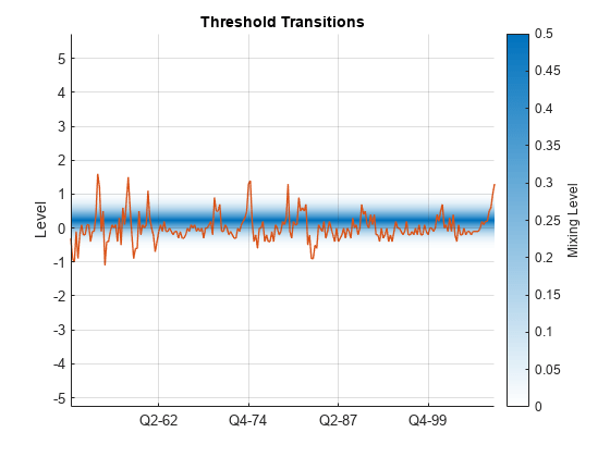
Display an estimation summary and plot the estimated switching mechanism with the threshold data.

summarize(EstMdl)

Description
1-Dimensional tsVAR Model with 2 Submodels

Switch
Transition Type: normal
Estimated Levels: 0.228
Estimated Rates: 3.000

Fit
Effective Sample Size: 237 
Number of Estimated Parameters: 4 
Number of Constrained Parameters: 6 
LogLikelihood: -267.892 
AIC: 543.784 
BIC: 557.656 

Submodels
                           Estimate     StandardError    TStatistic      PValue  
                           _________    _____________    __________    __________

    State 1 Constant(1)       1.5928      0.087805           18.14      1.543e-73
    State 1 AR{1}(1,1)             0             0             NaN            NaN
    State 1 AR{2}(1,1)             0             0             NaN            NaN
    State 1 AR{3}(1,1)             0             0             NaN            NaN
    State 1 AR{4}(1,1)      -0.11789      0.067607         -1.7438       0.081194
    State 2 Constant(1)     -0.73667       0.15808         -4.6601     3.1609e-06
    State 2 AR{1}(1,1)             0             0             NaN            NaN
    State 2 AR{2}(1,1)             0             0             NaN            NaN
    State 2 AR{3}(1,1)             0             0             NaN            NaN
    State 2 AR{4}(1,1)     -0.040337        0.1299        -0.31053        0.75616

figure
ttplot(EstMdl.Switch,Data=gUNRATE(idxEst))
dEst = dates(idxEst);
xticklabels(string(dEst(xticks)))

Estimate Model Containing Regression Component

Consider the following data-generating process (DGP) for a 2-D time-varying TAR (TVTAR) model containing an exogenous regression component.

• State 1: $$y_t=\left[\begin{array}{c}1\\ -1\end{array}\right]+\left[\begin{array}{cc}0.6& 0.1\\ 0.4& 0.2\end{array}\right]y_{t-1}+x_t\left[\begin{array}{c}0.2\\ -0.4\end{array}\right]+{\epsilon }_{1,t}$$, where ${\epsilon }_{1,\mathit{t}}\sim {{\rm N}}_2\left(0,0.5{\mathit{I}}_2\right)$ and ${\mathit{I}}_2$ is the 2-by-2 identity matrix.

• State 2: $$y_t=\left[\begin{array}{c}2\\ -2\end{array}\right]+\left[\begin{array}{cc}0.6& 0.1\\ 0.4& 0.2\end{array}\right]y_{t-1}+x_t\left[\begin{array}{c}0.6\\ -1.0\end{array}\right]+{\epsilon }_{2,t}$$, where ${\epsilon }_{2,\mathit{t}}\sim {{\rm N}}_2\left(0,{\mathit{I}}_2\right)$.

• State 3: $$y_t=\left[\begin{array}{c}3\\ -3\end{array}\right]+\left[\begin{array}{cc}0.6& 0.1\\ 0.4& 0.2\end{array}\right]y_{t-1}+x_t\left[\begin{array}{c}0.9\\ -1.3\end{array}\right]+{\epsilon }_{3,t}$$, where ${\epsilon }_{3,\mathit{t}}\sim {{\rm N}}_2\left(0,1.5{\mathit{I}}_2\right)$.

• The exogenous threshold variable ${\mathit{z}}_{\mathit{t}}$ represents a linear time trend over the sample period. In this example, ${\mathit{z}}_{\mathit{t}}$ is the sampling period normalized by the sample size.

• The system is in state 1 when ${\mathit{z}}_{\mathit{t}}<0.3$, the system is in state 2 when $0.3\le {\mathit{z}}_{\mathit{t}}<0.6$, and the system is in state 3 otherwise.

Create a TVTAR model that represents the DGP.

tDGP = [0.3 0.6];
ttDGP = threshold(tDGP);

% Constant vectors
C1 = [1;-1];
C2 = [2;-2];
C3 = [3;-3];

% Common Autoregression coefficient
AR = {[0.6 0.1; 0.4 0.2]};

% Regression coefficient vectors
Beta1 = [0.2;-0.4];
Beta2 = [0.6;-1.0];
Beta3 = [0.9;-1.3];

% Innovations covariance matrices
Sigma1 = 0.5*eye(2);
Sigma2 = eye(2);
Sigma3 = 1.5*eye(2);

% VAR Submodels
mdl1 = varm(Constant=C1,AR=AR,Beta=Beta1,Covariance=Sigma1);
mdl2 = varm(Constant=C2,AR=AR,Beta=Beta2,Covariance=Sigma2);
mdl3 = varm(Constant=C3,AR=AR,Beta=Beta3,Covariance=Sigma3);
mdlDGP = [mdl1; mdl2; mdl3];

DGP = tsVAR(ttDGP,mdlDGP);

For the exogenous predictors ${\mathit{x}}_{\mathit{t}}$, simulate a 2-D 1000-period path from the Gaussian distribution with mean 0 and standard deviation 10.

rng(1); % For reproducibility
numPeriods = 1000;
X = 10*randn(numPeriods,2);

For the threshold variable, create a 1000-element vector of equally spaced elements from 0 to 1.

z = linspace(0,1,numPeriods)';

Simulate a 1000-period path from the DGP.

Y = simulate(DGP,numPeriods,X=X,Type="exogenous",Z=z);

Create a TVTAR model template for estimation. Specify all estimable parameters as unknown by using NaNs.

t = [NaN NaN];
tt = threshold(t);

mdl = varm(2,1);        % Unknown contsant and AR coefficient by default
mdl.Beta = NaN(2,1);    % Configure exogenous regression component for estimation
Mdl = tsVAR(tt,[mdl; mdl; mdl]);

Specify initial values of 0.25 and 0.7 for the regime thresholds.

t0 = [.25 .7];
tt0 = threshold(t0);

The largest lag among all models is 1. Therefore, the estimation procedure requires one presample observation to initialize the model.

Identify indices for the required presample, and identify indices for the estimation sample.

p = mdl.P;
idxPre = 1:p;
idxEst = (p + 1):numPeriods;

Fit the TVTAR model to the data. Specify presample responses Y0, characterize the threshold variable Type and provide its data Z, and specify the exogenous data X.

EstMdl = estimate(Mdl,tt0,Y(idxEst,:),Y0=Y(idxPre,:), ...
    Type="exogenous",Z=z(idxEst),X=X(idxEst,:));

Display an estimation summary separately for each state, and display the estimated threshold transitions.

summarize(EstMdl,1)

Description
2-Dimensional VAR Submodel, State 1

Submodel
                           Estimate    StandardError    TStatistic      PValue   
                           ________    _____________    __________    ___________

    State 1 Constant(1)      0.6284        0.1463         4.2952       1.7456e-05
    State 1 Constant(2)    -0.86147        0.1664        -5.1771       2.2538e-07
    State 1 AR{1}(1,1)      0.64569      0.046378         13.922       4.6483e-44
    State 1 AR{1}(2,1)      0.41777      0.052749           7.92       2.3752e-15
    State 1 AR{1}(1,2)      0.11447      0.029747         3.8481       0.00011901
    State 1 AR{1}(2,2)      0.18968      0.033833         5.6064       2.0657e-08
    State 1 Beta(1,1)       0.12661       0.01005         12.598       2.1562e-36
    State 1 Beta(2,1)      -0.28306       0.01143        -24.765      2.1435e-135

summarize(EstMdl,2)

Description
2-Dimensional VAR Submodel, State 2

Submodel
                           Estimate    StandardError    TStatistic      PValue  
                           ________    _____________    __________    __________

    State 2 Constant(1)     2.0016        0.20741         9.6503      4.9029e-22
    State 2 Constant(2)     -1.919         0.2359        -8.1345      4.1377e-16
    State 2 AR{1}(1,1)     0.59692       0.033401         17.871      1.9848e-71
    State 2 AR{1}(2,1)     0.37274        0.03799         9.8117      1.0027e-22
    State 2 AR{1}(1,2)      0.1173       0.023148         5.0674      4.0337e-07
    State 2 AR{1}(2,2)     0.18002       0.026327         6.8376      8.0532e-12
    State 2 Beta(1,1)       0.6689       0.014264         46.896               0
    State 2 Beta(2,1)       -1.122       0.016223         -69.16               0

summarize(EstMdl,3)

Description
2-Dimensional VAR Submodel, State 3

Submodel
                           Estimate    StandardError    TStatistic      PValue   
                           ________    _____________    __________    ___________

    State 3 Constant(1)     3.1135         0.10796        28.841      6.5868e-183
    State 3 Constant(2)     -3.135         0.12279       -25.533      8.5619e-144
    State 3 AR{1}(1,1)     0.61547        0.011379        54.089                0
    State 3 AR{1}(2,1)     0.40065        0.012942        30.958      1.9801e-210
    State 3 AR{1}(1,2)     0.10685       0.0089014        12.004       3.4042e-33
    State 3 AR{1}(2,2)     0.19124        0.010124        18.889       1.3979e-79
    State 3 Beta(1,1)      0.92011       0.0080742        113.96                0
    State 3 Beta(2,1)      -1.3378       0.0091834       -145.68                0

EstMdl.Switch

ans = 
  threshold with properties:

          Type: 'discrete'
        Levels: [0.3096 0.5887]
         Rates: []
    StateNames: ["1"    "2"    "3"]
     NumStates: 3

Input Arguments

Mdl — Partially specified threshold-switching dynamic regression model

tsVAR model object

Partially specified threshold-switching dynamic regression model used to indicate constrained and estimable model parameters, specified as a tsVAR model object returned by tsVAR. Properties of Mdl describe the model structure and specify the parameters.

estimate treats specified parameters as equality constraints during estimation.

estimate fits unspecified (NaN-valued) parameters to the data Y.

Because estimate computes innovations covariances after estimation, you cannot constrain them. If Mdl.Covariance is nonempty (see tsVAR), estimate provides an estimate in EstMdl.Covariance. Otherwise, for each i in 1:Mdl.NumStates, estimate provides the innovations covariance estimate of state i in EstMdl.Submodels(i).Covariance.

tt0 — Fully specified threshold transitions

threshold object

Fully specified threshold transitions used to initialize the estimation procedure, specified as a threshold object returned by threshold. Properties of a fully specified model object do not contain NaN values.

tt0 is a copy of Mdl.Switch with NaN values replaced by initial values for levels (Mdl.Switch.Levels) and rates (Mdl.Switch.Rates). Levels (tt0.Levels) and rates (tt0.Rates) must be within the limits set by the name-value arguments 'MaxLevel' and 'MaxRate'.

Tip

For broad coverage of the parameter space, run the algorithm from multiple instances of tt0. For more details, see Algorithms.

Y — Observed response data

numeric matrix

Observed response data to which estimate fits the model, specified as a numObs-by-numSeries numeric matrix.

numObs is the sample size. numSeries is the number of response variables (Mdl.NumSeries).

Rows correspond to observations, and the last row contains the latest observation. Columns correspond to individual response variables.

Y represents the continuation of the presample response series in Y0.

Data Types: double

ax — Axes on which to plot loglikelihood for each iteration

Axes object

Axes on which to plot the loglikelihood for each iteration when the 'IterationPlot' name-value argument is true, specified as an Axes object.

By default, estimate plots to the current axes (gca).

If 'IterationPlot' is false, estimate ignores ax.

Name-Value Arguments

Specify optional pairs of arguments as Name1=Value1,...,NameN=ValueN, where Name is the argument name and Value is the corresponding value. Name-value arguments must appear after other arguments, but the order of the pairs does not matter.

Before R2021a, use commas to separate each name and value, and enclose Name in quotes.

Example: Type="exogenous",Z=z,IterationPlot=true specifies data z for the exogenous threshold variable and plots the loglikelihood for each iteration.

Type — Type of threshold variable data

"endogenous" (default) | "exogenous"

Type of threshold variable data, specified as a value in this table.

Value	Description
"endogenous"	The model is self-exciting with threshold variable data $$z_t=y_{j,(t-d)},$$ generated by response j, where The name-value argument 'Delay' specifies the delay d. The name-value argument 'Index' specifies the component j of the multivariate response variable.
"exogenous"	The threshold variable is exogenous to the system. The name-value argument 'Z' specifies the threshold variable data and is required.

Example: Type="exogenous",Z=z specifies the data z for the exogenous threshold variable.

Example: Type="endogenous",Index=2,Delay=4 specifies the endogenous threshold variable as y_2,t−4, whose data is Y(:,2).

Data Types: char | string | cell

Y0 — Presample response data

numeric matrix

Presample response data, specified as a numPreSampleObs-by-numSeries numeric matrix.

The number of presample observations numPreSampleObs must be sufficient to initialize the AR terms of all submodels. For models of type "endogenous", the number of presample observations must also be sufficient to initialize the delayed response. If numPreSampleObs exceeds the number necessary to initialize the model, estimate uses only the latest observations. The last row contains the latest observations.

By default, Y0 is the initial segment of Y, which reduces the effective sample size.

Data Types: double

Z — Threshold variable data z_t

[] (default) | numeric vector

Threshold variable data for models of type "exogenous", specified as a numeric vector of length at least numObs. If the length exceeds numobs, estimate uses only the latest observations. The last row contains the latest observation.

Data Types: double

Delay — Threshold variable delay d in y_j,t−d

1 (default) | positive integer

Threshold variable delay d in y_j,t−d, for models of type "endogenous", specified as a positive integer.

Example: Delay=4 specifies that the threshold variable is y_2,t−d, where j is the value of Index

.

Data Types: double

Index — Threshold variable index j in y_j,t−d

1 (default) | scalar in 1:Mdl.NumSeries

Threshold variable index j in y_j,t−d for models of type "endogenous", specified as a scalar in 1:Mdl.NumSeries.

estimate ignores Index for univariate AR models.

Example: Index=2 specifies that the threshold variable is y_2,t−d, where d is the value of Delay.

Data Types: double

X — Predictor data

numeric matrix | cell vector of numeric matrices

Predictor data used to evaluate regression components in all submodels of Mdl, specified as a numeric matrix or a cell vector of numeric matrices.

To use a subset of the same predictors in each state, specify X as a matrix with numPreds columns and at least numObs rows. Columns correspond to distinct predictor variables. Submodels use initial columns of the associated matrix, in order, up to the number of submodel predictors. The number of columns in the Beta property of Mdl.SubModels(j) determines the number of exogenous variables in the regression component of submodel j. If the number of rows exceeds numObs, then estimate uses the latest observations.

To use different predictors in each state, specify a cell vector of such matrices with length numStates.

By default, estimate ignores regression components in Mdl.

Data Types: double

MaxLevel — Maximum deviation of estimated threshold levels

0 (default) | positive numeric scalar

Maximum deviation of estimated threshold levels above or below the threshold variable data, z or y_j,t−d, specified as a positive numeric scalar representing the percent of the range.

The default value 0 means that initial and estimated levels must be within the range of the data. A value greater than 0 expands the range of the search.

Example: MaxLevel=10 expands the search for levels 10% above and below the range of the threshold variable data.

Data Types: double

MaxRate — Maximum estimated threshold transition rates

positive numeric scalar | positive numeric vector

Maximum estimated threshold transition rates, specified as a positive numeric scalar or vector with length equal to the number of rates in Mdl.Switch.Rates.

For a scalar, all estimated rates are bounded by MaxRate. For a vector, the estimate of Mdl.Switch.Rate(j) is bounded by MaxRate(j).

estimate estimates discrete transition levels as logistic transitions at MaxRate.

The default value is 10 for each rate.

Example: MaxLevel=3 bounds all estimated rates in Mdl.Switch.Rates by 3.

Example: MaxLevel=[5 10] bounds Mdl.Switch.Rates(1) by 5 and bounds Mdl.Switch.Rates(2) by 10.

Data Types: double

MaxItertations — Limit on number of iterations of threshold search algorithm

100 (default) | positive integer

Limit on the number of iterations of the threshold search algorithm, specified as a positive integer.

Example: MaxIterations=1000

Data Types: double

Tolerance — Convergence tolerance

1e-6 (default) | positive numeric scalar

Convergence tolerance, specified as a positive numeric scalar. The search algorithm terminates after an iteration in which the optimality tolerance on loglikelihood objective logL changes by less than the value of Tolerance.

Example: Tolerance=1e-4

Data Types: double

IterationPlot — Flag indicating whether to show plot of loglikelihood versus iteration step

false (default) | true

Flag indicating whether to show a plot of the loglikelihood versus iteration step at algorithm termination, specified as a value in this table.

Value	Description
true	When the algorithm terminates, estimate shows a plot of the loglikelihood at each iteration step.
false	estimate does not show a plot.

Example: IterationPlot=true

Data Types: logical

Output Arguments

EstMdl — Estimated threshold-switching dynamic regression model

tsVAR object

Estimated threshold-switching dynamic regression model, returned as a tsVAR object. EstMdl is a copy of Mdl that has NaN values replaced with parameter estimates. EstMdl is fully specified.

logL — Estimated loglikelihood

numeric scalar

Estimated loglikelihood of the data in Y from the conditional least-squares problem, returned as a numeric scalar and evaluated at the optimal parameter values in the threshold transitions EstMdl.Switch. For more details, see Algorithms.

h — Handle to iteration plot

graphics object

Handle to the iteration plot, returned as a graphics object when IterationPlot is true.

h contains a unique plot identifier, which you can use to query or modify properties of the plot.

Tips

• Several factors can lead to poor estimates of model parameters. The factors include:

  • Threshold data does not cross levels or sufficiently sample submodels.

  • Mdl contains more estimable parameters than the sample size supports.

  • High-rate transitions are indistinguishable.

  • Self-exciting autoregressive models have multiple sources of endogenous dynamics.

  To improve estimates, perform these actions:

  • Control the parameter search by experimenting with the 'MaxLevel' and 'MaxRate' name-value arguments.

  • Consider a parsimonious model with initial levels within the range of threshold variable data.

  • Constrain specific parameters to potentially improve performance.

• To estimate the delay d in a self-exciting model, compare the loglikelihood logL with different specifications for the 'Delay' name-value argument. In practice, usually d is limited to a range of reasonable values.

• You can estimate a simple time-varying STAR (TVSTAR) model by specifying exogenous threshold data z = t, which is a linear time trend over the sample period [3].

Algorithms

• estimate searches over levels and rates for EstMdl.Switch while solving a conditional least-squares problem for submodel parameters, maximizing the data likelihood, as described in [4]. logL is conditional on the optimal parameter values in EstMdl.Switch.

• Models with smooth transitions (STAR models) represent the response as a weighted mixture of conditional means from all submodels ([4], Eqn. 3.6). estimate determines the weights by the value of the threshold variable, z or y_j,t−d, relative to threshold levels. estimate treats models with discrete transitions (TAR models) as logistic STAR models with transition rates set to 'MaxRate' in order to disambiguate search levels that fall between threshold variable data.

• estimate handles two types of equality constraints.

  • Constraints on threshold transition levels and rates are enforced by fmincon during the search procedure.

  • Constraints on submodel parameters are enforced by the estimate function of the varm object at each search iteration.

  estimate computes innovations variances and covariances after estimation. Therefore, you cannot constrain them.

References

[1] Chan, Kung-Sik, and Howell Tong. “On Estimating Thresholds in Autoregressive Models.” Journal of Time Series Analysis 7 (May 1986): 179–90. https://doi.org/10.1111/j.1467-9892.1986.tb00501.x.

[2] Hamilton, James D. Time Series Analysis. Princeton, NJ: Princeton University Press, 1994.

[3] Teräsvirta, Tima. "Modelling Economic Relationships with Smooth Transition Regressions." In A. Ullahand and D.E.A. Giles (eds.), Handbook of Applied Economic Statistics, 507–552. New York: Marcel Dekker, 1998.

[4] van Dijk, Dick. Smooth Transition Models: Extensions and Outlier Robust Inference. Rotterdam, Netherlands: Tinbergen Institute Research Series, 1999.

Version History

Introduced in R2021b