Simulate VAR Model Conditional Responses
This example shows how to generate simulated responses in the forecast horizon when some of the response values are known. To illustrate conditional simulation generation, the example models quarterly measures of the consumer price index (CPI) and the unemployment rate as a VAR(4) model.
Load the Data_USEconModel data set.
load Data_USEconModelPlot the two series on separate plots.
figure
plot(DataTimeTable.Time,DataTimeTable.CPIAUCSL);
title('Consumer Price Index')
ylabel('Index')
xlabel('Date')
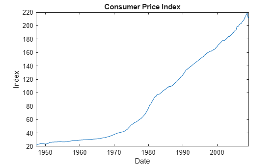
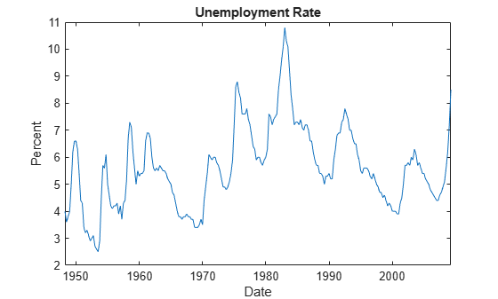
figure
plot(DataTimeTable.Time,DataTimeTable.UNRATE);
title('Unemployment Rate')
ylabel('Percent')
xlabel('Date')
The CPI appears to grow exponentially.
Stabilize the CPI by converting it to a series of growth rates. Synchronize the two series by removing the first observation from the unemployment rate series. Create a new data set containing the transformed variables, and do not include any rows containing at least one missing observation.
rcpi = price2ret(DataTimeTable.CPIAUCSL);
unrate = DataTimeTable.UNRATE(2:end);
Data = array2timetable([rcpi unrate],'RowTimes',DataTimeTable.Time(2:end),...
    'VariableNames',{'rcpi','unrate'});
Create a default VAR(4) model using shorthand syntax.
Mdl = varm(2,4)
Mdl =
  varm with properties:

     Description: "2-Dimensional VAR(4) Model"
     SeriesNames: "Y1"  "Y2"
       NumSeries: 2
               P: 4
        Constant: [2×1 vector of NaNs]
              AR: {2×2 matrices of NaNs} at lags [1 2 3 ... and 1 more]
           Trend: [2×1 vector of zeros]
            Beta: [2×0 matrix]
      Covariance: [2×2 matrix of NaNs]
Mdl is a varm model object. It serves as a template for model estimation.
Fit the model to the data.
EstMdl = estimate(Mdl,Data.Variables)
EstMdl =
  varm with properties:

     Description: "AR-Stationary 2-Dimensional VAR(4) Model"
     SeriesNames: "Y1"  "Y2"
       NumSeries: 2
               P: 4
        Constant: [0.00171639 0.316255]'
              AR: {2×2 matrices} at lags [1 2 3 ... and 1 more]
           Trend: [2×1 vector of zeros]
            Beta: [2×0 matrix]
      Covariance: [2×2 matrix]
EstMdl is a varm model object. EstMdl is structurally the same as Mdl, but all parameters are known.
Suppose that an economist expects the unemployment rate to remain the same as the last observed rate for the next two years. Create an 8-by-2 matrix in which the first column contains NaN values and the second column contains the last observed unemployment rate.
YF = [nan(8,1) repmat(Data.unrate(end),8,1)];
Using the estimated model, simulate 1000 paths of the quarterly CPI growth rate for the next two years. Assume that the unemployment rate remains the same for the next two years. Specify the entire data set as presample observations and the known values in the forecast horizon.
numpaths = 1000;
rng(1); % For reproducibility
Y = simulate(EstMdl,8,'Y0',Data.Variables,'NumPaths',numpaths,'YF',YF);
Y is an 8-by-2-by-1000 array of response paths. Although the first column on each page contains simulated values, the second column consists entirely of the last observed unemployment rate.
Estimate the average CPI growth rate at each point in the forecast horizon.
MCForecast = mean(Y,3)
MCForecast = 8×2

   -0.0075    8.5000
   -0.0134    8.5000
   -0.0010    8.5000
   -0.0050    8.5000
   -0.0052    8.5000
   -0.0022    8.5000
   -0.0032    8.5000
   -0.0026    8.5000
Given that the unemployment rate is 8.5 for the next two years, the CPI growth rate is expected to shrink.