Perform Outlier Detection Using Bayesian Non-Gaussian State-Space Models
This example shows how to use non-Gaussian error distributions in a Bayesian state-space model to detect outliers in a time series. The example follows the state-space framework for outlier detection in [1], Chapter 14.
Robust regressions that employ distributions with excess kurtosis accommodate more extreme data compared to the Gaussian regressions. After a non-Gaussian regression (representing, for example, a linear time series decomposition model), an analysis of residuals (representing the irregular component of the decomposition) facilitates outlier detection.
Consider using a state-space model as a linear filter for a simulated, quarterly series of coal consumption, in millions of short tons, from 1994 through 2020.
Load and Plot Data
Load the simulated coal consumption series Data_SimCoalConsumption.mat. The data set contains the timetable of data DataTimeTable.
load Data_SimCoalConsumptionPlot the coal consumption series.
figure
plot(DataTimeTable.Time,DataTimeTable.CoalConsumption)
ylabel("Consumption (Millions of Short Tons)")
title("Quarterly Coal Consumption, 1994-2020")
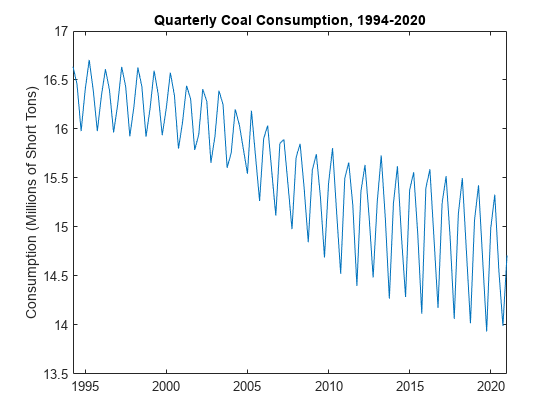
The series has a clear downward trend and pronounced seasonality, which suggests a linear decomposition model. The series does not explicitly exhibit unusually large or small observations.
Specify State-Space Model Structure
Because the series appears decomposable, consider the linear decomposition for the observed series , where, at time :
is the observed coal consumption.
is the unobserved local linear trend.
is the unobserved seasonal component.
is the observation innovation with mean 0. Its standard deviation depends on its distribution.
is the observation innovation coefficient, an unknown parameter, which scales the observation innovation.
The unobserved components are the model states, explicitly:
At time :
and are state disturbance series with mean 0. Their standard deviations depend on its distribution.
and are the state-disturbance loading scalars, which are unknown parameters.
Rearrange the linear trend equation to obtain .
The structure can be viewed as a state-space model
,
where:
, where are dummy variables for higher order lagged terms of and .
.
.
.
.
Write a function called linearDecomposeMap in the Local Functions section that maps a vector of parameters to the state-space coefficient matrices.
function [A,B,C,D,Mean0,Cov0,StateType] = linearDecomposeMap(theta)
    A = [2 -1  0  0  0;
         1  0  0  0  0;
         0  0 -1 -1 -1;
         0  0  1  0  0;
         0  0  0  1  0];
    B = [theta(1) 0; 0 0; 0 theta(2); 0 0; 0 0];
    C = [1 0 1 0 0];
    D = theta(3);
    Mean0 = [];         % MATLAB uses default initial state mean
    Cov0 = [];          % MATLAB uses initial state covariances
    StateType = [2; 2; 2; 2; 2]; % All states are nonstationary
end
Specify Prior Distribution
Assume the prior distribution of each of the disturbance and innovation scalars is . Write a function called priorDistribution in the Local Functions section that returns the log prior of a value of .
function logprior = priorDistribution(theta)
    p = chi2pdf(theta,10);
    logprior = sum(log(p));
end
Create Bayesian State-Space Model
Create a Bayesian state-space model representing the system by passing the state-space model structure and prior distribution functions as function handles to bssm. For comparison, create a model that sets the distribution of to a standard Gaussian distribution and a different model that sets the distribution of to a Student's distribution with unknown degrees of freedom.
y = DataTimeTable.CoalConsumption;
MdlGaussian = bssm(@linearDecomposeMap,@priorDistribution);
MdlT = bssm(@linearDecomposeMap,@priorDistribution,ObservationDistribution="t");
Prepare for Posterior Sampling
Posterior sampling requires a good set of initial parameter values and tuned proposal scale matrix. Also, to access Bayesian estimates of state values and residuals, which compose the components of the decomposition, you must write a function that stores these quantities at each iteration of the MCMC sampler.
For each prior model, use the tune function to obtain a data-driven set of initial values and a tuned proposal scale matrix. Specify a random set of positive values in [0,1] to initialize the Kalman filter.
rng(10)  % For reproducibility
numParams = 3;
theta0 = rand(numParams,1);
[theta0Gaussian,ProposalGaussian] = tune(MdlGaussian,y,theta0,Display=false);
Local minimum possible. fminunc stopped because it cannot decrease the objective function along the current search direction. <stopping criteria details>
[theta0T,ProposalT] = tune(MdlT,y,theta0,Display=false);
Local minimum possible.

fminunc stopped because it cannot decrease the objective function
along the current search direction.

<stopping criteria details>
Write a function in the Local Functions section called outputfcn that returns state estimates and observation residuals at each iteration of the MCMC sampler.
function out = outputfcn(inputstruct)
    out.States = inputstruct.States;
    out.ObsResiduals = inputstruct.Y - inputstruct(end).States*inputstruct(end).C';
end
Decompose Series Using Gaussian Model
Decompose the series by following this procedure:
Draw a large sample from the posterior distribution by using
simulate.Plot the linear, seasonal, and irregular components.
Use simulate to draw a posterior sample of 10000 from the model that assumes the observation innovation distribution is Gaussian. Specify the data-driven initial values and proposal scale matrix, specify the output function outputfcn, apply the univariate treatment to speed up calculations, and apply a burn-in period of 1000. Return the draws, acceptance probability, and output function output. simulate uses the Metropolis-Hastings sampler to draw the sample.
NumDraws = 10000;
BurnIn = 1000;
[ThetaPostGaussian,acceptGaussian,outGaussian] = simulate(MdlGaussian, ...
    y,theta0Gaussian,ProposalGaussian,NumDraws=NumDraws,BurnIn=BurnIn, ...
    OutputFunction=@outputfcn,Univariate=true);
acceptGaussian
acceptGaussian =
0.4603
ThetaPostGaussian is a 3-by-1000 matrix of draws from the posterior distribution of . simulate accepted about half of the proposed draws. outGaussian is a structure array with 1000 records, the last of which contains the final estimates of the components of the decomposition.
Plot the components of the decomposition by calling the plotComponents function in the Local Functions section.
plotComponents(outGaussian,dates,"Gaussian")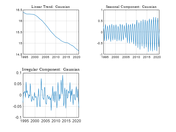
The plot of the irregular component (residuals) does not contain any residuals of unusual magnitude. Because the Gaussian model structure applies very small probabilities to unusual observations, it is difficult for this type of model to discover outliers.
Decompose Series Using Model with t-Distributed Innovations
The -distribution applies larger probabilities to extreme observations. This characteristic enables models to discover outliers more readily than a Gaussian model.
Decompose the series by following this procedure:
Estimate the posterior distribution by using
estimate. Inspect the estimate of .Draw a large sample from the posterior distribution by using
simulate.Plot the linear, seasonal, and irregular components.
Estimate the posterior distribution of the model that assumes the observation innovations are distributed.
seed = 10; % To reproduce samples across estimate and simulate
rng(seed)
estimate(MdlT,y,theta0T,NumDraws=NumDraws,BurnIn=BurnIn,Univariate=true);
Local minimum possible.
fminunc stopped because it cannot decrease the objective function
along the current search direction.
<stopping criteria details>
Optimization and Tuning
| Params0 Optimized ProposalStd
----------------------------------------
c(1) | 0.0035 0.0035 0.0011
c(2) | 0.0620 0.0620 0.0081
c(3) | 0.0392 0.0392 0.0096
Posterior Distributions
| Mean Std Quantile05 Quantile95
--------------------------------------------------
c(1) | 0.0042 0.0013 0.0025 0.0067
c(2) | 0.0502 0.0069 0.0395 0.0622
c(3) | 0.0266 0.0074 0.0159 0.0399
x(1) | 14.6301 0.0304 14.5801 14.6795
x(2) | 14.6540 0.0241 14.6146 14.6938
x(3) | 0.1210 0.0508 0.0516 0.2173
x(4) | -0.6856 0.0381 -0.7548 -0.6328
x(5) | -0.1140 0.0310 -0.1638 -0.0638
ObsDoF | 2.5304 0.7753 1.5634 4.1030
Proposal acceptance rate = 30.59%
The Posterior Distributions table in the display shows posterior estimates of the state-space model parameters (labeled c(j)), final state values (labeled x(j)), and -distribution degrees of freedom (labeled ObsDoF). The posterior mean of the degrees of freedom is about 5, which is low. This result suggests that the observation innovations have excess kurtosis.
Use simulate to draw a posterior sample of 10000 from the model that assumes the observation innovations are distributed. Specify the data-driven initial values and proposal scale matrix, specify the output function outputfcn, apply the univariate treatment to speed up calculations, and apply a burn-in period of 1000. Return the draws, acceptance probability, and output function output. simulate uses the Metropolis-within-Gibbs sampler to draw the sample.
rng(seed)
[ThetaPostT,acceptT,outT] = simulate(MdlT,y,theta0T,ProposalT, ...
    NumDraws=NumDraws,BurnIn=BurnIn,OutputFunction=@outputfcn,Univariate=true);
acceptT
acceptT = 0.3388
ThetaPostT is a 3-by-1000 matrix of draws from the posterior distribution of . simulate accepted about 30% of the proposed draws. outT is a structure array with 1000 records, the last of which contains the final estimates of the components of the decomposition.
Plot the components of the decomposition.
plotComponents(outT,dates,"$$t$$")
h = gca;
h.FontSize = 8;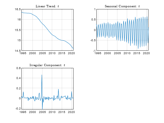
The plot of the irregular component shows two clear outliers around 2005.
Local Functions
This example uses the following functions. linearDecomposeMap is the parameter-to-matrix mapping function and priorDistribution is the log prior distribution of the parameters .
function [A,B,C,D,Mean0,Cov0,StateType] = linearDecomposeMap(theta)
    A = [2 -1  0  0  0;
         1  0  0  0  0;
         0  0 -1 -1 -1;
         0  0  1  0  0;
         0  0  0  1  0];
    B = [theta(1) 0; 0 0; 0 theta(2); 0 0; 0 0];
    C = [1 0 1 0 0];
    D = theta(3);
    Mean0 = [];         % MATLAB uses default initial state mean
    Cov0 = [];          % MATLAB uses initial state covariances
    StateType = [2; 2; 2; 2; 2]; % All states are nonstationary
end

function logprior = priorDistribution(theta)
    p = chi2pdf(theta,10);
    logprior = sum(log(p));
end

function out = outputfcn(inputstruct)
    out.States = inputstruct.States;
    out.ObsResiduals = inputstruct.Y - inputstruct(end).States*inputstruct(end).C';
end

function plotComponents(output,dt,tcont)
    figure
    tiledlayout(2,2)
    nexttile
    plot(dt,output(end).States(:,1))
    grid on
    title("Linear Trend: " + tcont,Interpreter="latex")
    h = gca;
    h.FontSize = 8;
    nexttile
    plot(dt,output(end).States(:,3))
    grid on
    title("Seasonal Component: " + tcont,Interpreter="latex")
    h = gca;
    h.FontSize = 8;
    nexttile
    plot(dt,output(end).ObsResiduals)
    grid on
    title("Irregular Component: " + tcont,Interpreter="latex")
end