hpfilter
Hodrick-Prescott filter for trend and cyclical components
Syntax
Description
The hpfilter function applies the Hodrick-Prescott filter to
separate one or more time series into additive trend and cyclical components.
hpfilter optionally plots the series and trend component, with
cycles removed. The plot helps you select a smoothing parameter.
In addition to the Hodrick-Prescott filter, Econometrics Toolbox™ supports the Baxter-King (bkfilter),
Christiano-Fitzgerald (cffilter), and
Hamilton (hfilter)
filters.
[
returns tables or timetables containing variables for the trend and cyclical components
from applying the Hodrick-Prescott filter to each variable in the input table or
timetable. To select different variables to filter, use the
TTbl,CTbl] = hpfilter(Tbl)DataVariables name-value argument. (since R2022a)
[___] = hpfilter(___,
specifies options using one or more name-value arguments in
addition to any of the input argument combinations in previous syntaxes.
Name=Value)hpfilter returns the output argument combination for the
corresponding input arguments. For example,
hpfilter(Tbl,Smoothing=100,DataVariables=1:5) applies the
Hodrick-Prescott filter to the first five variables in the input table
Tbl and sets the smoothing parameter to
100. (since R2022a)
hpfilter(___) plots time series variables in the
input data and their respective trend components, computed by the Hodrick-Prescott filter,
on the same axes.
hpfilter(
plots on the axes specified by ax,___)ax instead of
the current axes (gca). ax can precede any of the input
argument combinations in the previous syntaxes. (since R2022a)
Examples
Plot the cyclical component of the US post-WWII, seasonally adjusted, quarterly, real gross national product (GNPR).
load Data_GNP
GNPR = Data(:,2);
[trend,cyclical] = hpfilter(GNPR);
T = numel(trend)
T = 235
trend and cyclical are 235-by-1 vectors containing the trend and cyclical components, respectively, resulting from applying the Hodrick-Prescott filter to the series with default smoothing parameter 1600.
plot(dates,cyclical)
axis tight
ylabel("Real GNP Cyclical Component")

Since R2022a
Apply the Hodrick-Prescott filter to all variables in input table variables.
Load the Schwert stock data set Data_SchwertStock.mat, which contains monthly returns of the NYSE index from 1871 through 2008 in DataTimeTableMth, among three other variables (for details, enter Description). Remove all missing observations from all series.
load Data_SchwertStock
TTM = rmmissing(DataTimeTableMth);
Aggregate the monthly data in the timetable to quarterly measurements.
TTQ = convert2quarterly(TTM);
Apply the Hodrick-Prescott filter to all variables in the quarterly timetable. The default smoothing parameter value is 1600. Display the last few observed components.
[TQTT,CQTT] = hpfilter(TTQ);
size(TQTT)
ans = 1×2

   220     4
tail(TQTT)
       Time         Return       DivYld        CapGain       CapGainA
    ___________    _________    _________    ___________    ___________

    31-Mar-1924    0.0046179    0.0067678     -0.0021499     -0.0021499
    30-Jun-1924     0.005586    0.0067204     -0.0011344     -0.0011344
    30-Sep-1924    0.0066431    0.0066689    -2.5812e-05    -2.5812e-05
    31-Dec-1924    0.0077772    0.0066142      0.0011629      0.0011629
    31-Mar-1925    0.0089687    0.0065574      0.0024113      0.0024113
    30-Jun-1925     0.010231    0.0064998      0.0037314      0.0037314
    30-Sep-1925     0.011543    0.0064423      0.0051005      0.0051005
    31-Dec-1925     0.012878    0.0063854      0.0064922      0.0064922
tail(CQTT)
       Time          Return        DivYld        CapGain       CapGainA
    ___________    __________    ___________    __________    __________

    31-Mar-1924     -0.019683     0.00033141     -0.020014     -0.020014
    30-Jun-1924      0.059151     5.7125e-05      0.059093      0.059093
    30-Sep-1924     -0.011788     0.00044598     -0.012234     -0.012234
    31-Dec-1924      0.052846     0.00052627       0.05232       0.05232
    31-Mar-1925     -0.056652    -0.00078018     -0.055872     -0.055872
    30-Jun-1925    -0.0069909     -0.0010415    -0.0059494    -0.0059494
    30-Sep-1925     0.0052352     -0.0011402     0.0063755     0.0063755
    31-Dec-1925      0.036713     0.00070754      0.036006      0.036006
TQTT and CQTT are 220-by-4 timetables containing the trend and cyclical components, respectively, of the series in TTQ. Variables in the input and output timetables correspond.
By default, hpfilter filters all variables in the input table or timetable. To select a subset of variables, set the DataVariables option.
To compare outputs between different tabular inputs, apply the Hodrick-Prescott filter to all variables in the table of monthly data DataTableMth and the timetable of monthly data TTM.
% Table input of daily data
DTM = rmmissing(DataTableMth);
[TMDT,CMDT] = hpfilter(DTM);
size(TMDT)
ans = 1×2
656 4
tail(TMDT)
                Return      DivYld      CapGain     CapGainA
               ________    _________    ________    ________

    May1925     0.02665    0.0045709    0.022079    0.022079
    Jun1925      0.0275     0.004558    0.022942    0.022942
    Jul1925    0.028372    0.0045491    0.023823    0.023823
    Aug1925     0.02926    0.0045437    0.024716    0.024716
    Sep1925    0.030152     0.004542     0.02561     0.02561
    Oct1925    0.031049     0.004543    0.026506    0.026506
    Nov1925    0.031941    0.0045461    0.027395    0.027395
    Dec1925    0.032844    0.0045508    0.028293    0.028293
tail(CMDT)
                 Return        DivYld       CapGain     CapGainA
               __________    __________    _________    _________

    May1925      0.039536    -0.0020878     0.041624     0.041624
    Jun1925      -0.02426    0.00090028     -0.02516     -0.02516
    Jul1925    -0.0095168    0.00066325     -0.01018     -0.01018
    Aug1925      0.018948    -0.0018318      0.02078      0.02078
    Sep1925     -0.013374    0.00076008    -0.014134    -0.014134
    Oct1925      0.037148    9.6588e-05     0.037051     0.037051
    Nov1925     -0.040405    -0.0017316    -0.038674    -0.038674
    Dec1925      0.016747     0.0025421     0.014205     0.014205
% Timetable input of daily data
[TMTT,CMTT] = hpfilter(TTM);
size(TMTT)
ans = 1×2
656 4
tail(TMTT)
       Time         Return      DivYld      CapGain     CapGainA
    ___________    ________    _________    ________    ________

    01-May-1925     0.02665    0.0045709    0.022079    0.022079
    01-Jun-1925      0.0275     0.004558    0.022942    0.022942
    01-Jul-1925    0.028372    0.0045491    0.023823    0.023823
    01-Aug-1925     0.02926    0.0045437    0.024716    0.024716
    01-Sep-1925    0.030152     0.004542     0.02561     0.02561
    01-Oct-1925    0.031049     0.004543    0.026506    0.026506
    01-Nov-1925    0.031941    0.0045461    0.027395    0.027395
    01-Dec-1925    0.032844    0.0045508    0.028293    0.028293
tail(CMTT)
       Time          Return        DivYld       CapGain     CapGainA
    ___________    __________    __________    _________    _________

    01-May-1925      0.039536    -0.0020878     0.041624     0.041624
    01-Jun-1925      -0.02426    0.00090028     -0.02516     -0.02516
    01-Jul-1925    -0.0095168    0.00066325     -0.01018     -0.01018
    01-Aug-1925      0.018948    -0.0018318      0.02078      0.02078
    01-Sep-1925     -0.013374    0.00076008    -0.014134    -0.014134
    01-Oct-1925      0.037148    9.6588e-05     0.037051     0.037051
    01-Nov-1925     -0.040405    -0.0017316    -0.038674    -0.038674
    01-Dec-1925      0.016747     0.0025421     0.014205     0.014205
Because the data is disaggregated, the outputs of the daily data have more rows than from the quarterly data. The filter results of the daily inputs are equal among the corresponding outputs, but hpfilter returns tables of results, instead of timetables, when you supply data in a table.
Since R2022a
Load the Nelson-Plosser macroeconomic data set Data_NelsonPlosser.mat, which contains series measured yearly in the table DataTable.
load Data_NelsonPlosserFilter the real and nominal GNP series, GNPR and GNPN, respectively. Plot the trend component with each series by additionally returning the vector of graphics objects. Set the smoothing parameter to 100, as suggested in [1] for yearly data.
[TTblHP,CTblHP,hHP] = hpfilter(DataTimeTable,Smoothing=100, ...
    DataVariables=["GNPR" "GNPN"]);

Filter the series again, but set the smoothing parameter to 6.25, which is the suggested smoothing parameter value in [3] for yearly data.
figure
[TTblRU,CTblRU,hRU] = hpfilter(DataTimeTable,Smoothing=6.25, ...
    DataVariables=["GNPR" "GNPN"]);

The smoothed trend of the latter plot contains more higher frequency cycles than the former plot, and, therefore, the smoothed trend in the latter plot follows the data more tightly.
Experiment with the smoothing parameter value by filtering the series several more times and setting the smoothing parameter to 0, 10, 100, 1000, 10,000, and Inf. Plot each set of results by not returning any outputs.
smoothing = [10.^(0:4) Inf];
tiledlayout(2,3)
for j = 1:numel(smoothing)
    nexttile
    hpfilter(DataTimeTable,Smoothing=smoothing(j), ...
        DataVariables=["GNPR" "GNPN"]);
    title("\lambda = " + string(smoothing(j)));
    legend("off")
end

Input Arguments
Name-Value Arguments
Output Arguments
More About
The Hodrick-Prescott filter decomposes an
observed time series yt (Y)
into a trend component τt
(Trend) and a cyclical component
ct (Cyclical) such that
yt =
τt +
ct. The method implements a high-pass filter for
the cycle that penalizes variations in the trend to a degree determined by the smoothing
parameter [1].
The objective function of the filter is
where:
T is the sample size.
λ is the smoothing parameter (
smoothing).yt – τt = ct.
The programming problem is to minimize the objective function over τ1,…,τT. The objective penalizes the sum of squares for the cyclical component with the sum of squares of second-order differences for the trend component (trend acceleration penalty). If λ = 0, the minimum of the objective is 0 with τt = yt for all t. As λ increases, the penalty for a flexible trend increases, resulting in an increasingly smoother trend. When λ is arbitrarily large, the trend acceleration approaches 0, resulting in a linear trend.
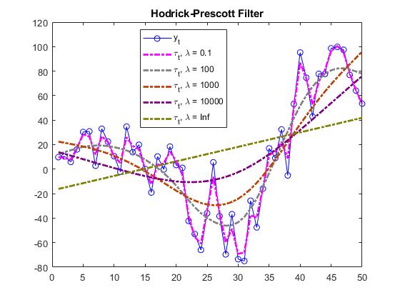
This figure shows the effects of increasing the smoothing parameter on the trend component for a simulated series.
The filter is equivalent to a cubic spline smoother, where the smoothed component is τt.
Tips
Hodrick and Prescott [1] suggest values for the smoothing parameter λ (
Smoothing) that depend upon the periodicity of the data, and Ravn and Uhlig [3] suggest adjustments to those values. This table contains their suggested smoothing parameter values for several data periodicities.Periodicity Hodrick and Prescott Suggested SmoothingRavn and Uhlig Suggested SmoothingYearly 100 6.25 Quarterly 1600 1600 Monthly 14400 129600 Supply a vector of smoothing parameters for the
Smoothingname-value argument to test alternatives. Plot the results to visually compare the alternatives.The default two-sided filter (see
FilterType) uses future values of the input series to compute outputs at time t. Because the filter is typically applied to historical data, the results can contain anomalous end effects unsuitable for forecasting [4]. The one-sided filter, by contrast, is causal because it uses only current and previous values of the input series. As a result, the one-sided filter does not revise outputs when new data becomes available.
Algorithms
hpfilter implements the closed-form solution in [2], Appendix A to the original Hodrick-Prescott programming problem [1].
Therefore, hpfilter requires complete data and removes
NaN values in the input data by using listwise deletion.
References
[1] Hodrick, Robert J., and Edward C. Prescott. "Postwar U.S. Business Cycles: An Empirical Investigation." Journal of Money, Credit and Banking 29, no. 1 (February 1997): 1–16. https://doi.org/10.2307/2953682.