Evaluate Threshold Transitions
This example shows how to evaluate transition functions and compute states of threshold transitions given transition variable data.
Evaluate Transition Functions
Consider defining discrete economic states based on the CPI-based Canadian inflation rate. Specifically:
Inflation is low when its rate is below 2%.
Inflation is moderate when its rate is at least 2% and below 8%.
Inflation is high when its rate is at least 8%.
Transitions are smooth and modeled using the logistic distribution.
The transition rate from low to moderate inflation is 3.5, and the rate from moderate to high inflation is 1.5.
Create threshold transitions representing the state space based on the CPI-based Canadian inflation rate. Assign names "Low", "Med", and "High" to the states.
ttL = threshold([2 8],Type="logistic",Rates=[3.5 1.5], ...
    StateNames=["Low" "Med" "High"]);
ttL is a threshold object that is a model for the state space of the inflation rate.
ttdata computes transition function data at specified values of a threshold variable .
Evaluate all transition functions of the inflation threshold transitions at the transition levels and 5.
z = [2 5 8];
F = ttdata(ttL,z)
F = 3×2

    0.5000    0.0001
    1.0000    0.0110
    1.0000    0.5000
F is a 3-by-2 matrix of transition function values. Its rows correspond to the threshold variable values z, and its columns correspond to the two transition functions at levels 2 and 8.
The UseZeroLevels name-value argument of ttdata evaluates transition functions relative to a zero level. This option is useful when you compare rates among the transition functions.
Illustrate comparing transition rates. Create threshold transitions, for an arbitrary threshold variable, at levels 0 and 5. Specify normal transition functions with rates 0.5 and 1.5. Create a grid of threshold data from -10 to 10.
ttN = threshold([0 5],Type="normal",Rates=[0.5 1.5]);
z = -10:0.01:10;
Evaluate each transition function for the threshold variable data. Compute raw values (UseZeroLevels=false) and values relative to level zero (UseZeroLevels=true).
F0 = ttdata(ttN,z,UseZeroLevels=false);
F1 = ttdata(ttN,z,UseZeroLevels=true);
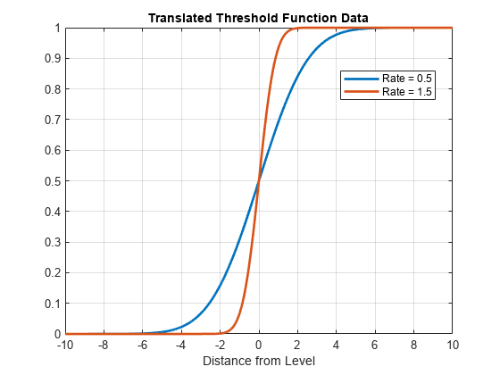
Separately plot each set of evaluated transition functions with respect to the transition function data.
figure
plot(z,F0,LineWidth=2)
grid on
xlabel("Level")
title("Raw Threshold Function Data")
legend(["Rate = 0.5" "Rate = 1.5"],Location="best")
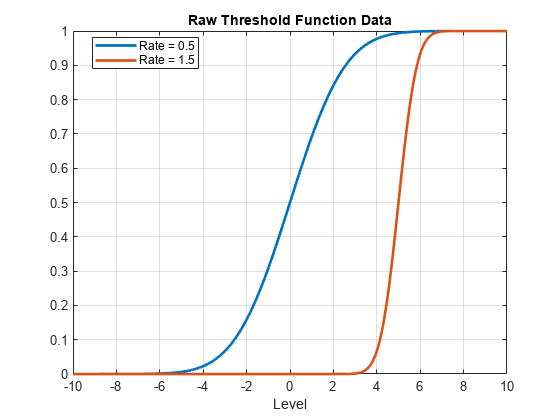
figure
plot(z,F1,LineWidth=2)
grid on
xlabel("Distance from Level")
title("Translated Threshold Function Data")
legend(["Rate = 0.5" "Rate = 1.5"],Location="best")
Use ttplot to reproduce the latter plot. Adjust the plot domain by specifying the Width name-value argument.
figure
ttplot(ttN,Type="graph",Width=20)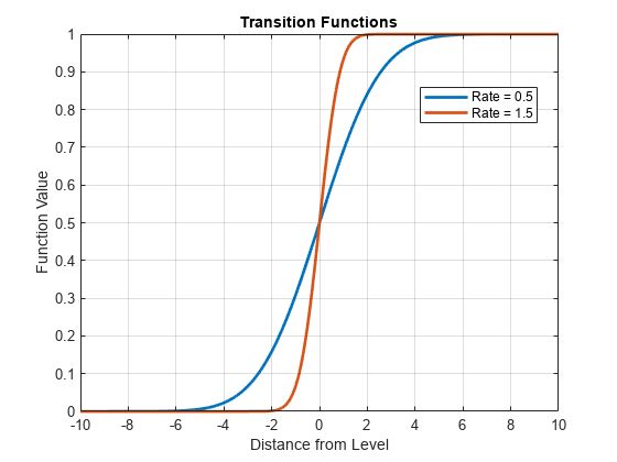
Compute States
ttstates computes the state path of threshold variable data relative to specified threshold levels.
Consider again the threshold transitions for the CPI-based Canadian inflation rate ttL. Load the data set Data_Canada.mat, which contains the inflation rate series INF_C.
load Data_Canada
INF_C = DataTable.INF_C;    % Inflation rate (threshold variable)
Determine the inflation state at each sample time point in the data by passing the threshold transitions and observed inflation rate series to ttstates. Display the first five states.
states = ttstates(ttL,INF_C);
sp15 = ttL.StateNames(states(1:5))'  % First five states
sp15 = 5×1 string
"Low"
"Low"
"Low"
"Med"
"Med"
Inflation is low for the first three observations, then the process crosses the first mid-level to moderate inflation for observations 4 and 5.
Visualize the entire state path.
figure
subplot(2,1,1)
ttplot(ttL,Data=INF_C)
colorbar('off')

subplot(2,1,2)
plot(states,"mo")
ylabel("State")
yticks([1 2 3])
yticklabels(ttL.StateNames)
axis tight
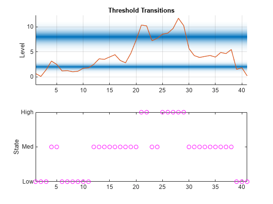
State transitions occur when the threshold variable crosses a transition mid-level. For TAR models, this results in an abrupt shift in the submodel computing the response. For STAR models, state changes indicate a shift in the dominant submodel in the mixture of submodel responses.