forecast
Forecast responses of Bayesian linear regression model
Syntax
Description
yF = forecast(Mdl,XF)numPeriods forecasted responses from the Bayesian linear regression
model
Mdl given the predictor data in XF, a
matrix with numPeriods rows.
To estimate the forecast, forecast uses the mean of
the numPeriods-dimensional posterior predictive distribution.
NaNs in the data indicate missing values, which
forecast removes using list-wise deletion.
yF = forecast(Mdl,XF,X,y)X and corresponding response
data y.
If
Mdlis a joint prior model, thenforecastproduces the posterior predictive distribution by updating the prior model with information about the parameters that it obtains from the data.If
Mdlis a posterior model, thenforecastupdates the posteriors with information about the parameters that it obtains from the additional data. The complete data likelihood is composed of the additional dataXandy, and the data that createdMdl.
yF = forecast(___,Name,Value)
Examples
Consider the multiple linear regression model that predicts the US real gross national product (GNPR) using a linear combination of industrial production index (IPI), total employment (E), and real wages (WR).
For all , is a series of independent Gaussian disturbances with a mean of 0 and variance .
Assume these prior distributions:
. is a 4-by-1 vector of means, and is a scaled 4-by-4 positive definite covariance matrix.
. and are the shape and scale, respectively, of an inverse gamma distribution.
These assumptions and the data likelihood imply a normal-inverse-gamma conjugate model.
Create a normal-inverse-gamma conjugate prior model for the linear regression parameters. Specify the number of predictors p and the variable names.
p = 3;
VarNames = ["IPI" "E" "WR"];
PriorMdl = bayeslm(p,'ModelType','conjugate','VarNames',VarNames);
Mdl is a conjugateblm Bayesian linear regression model object representing the prior distribution of the regression coefficients and disturbance variance.
Load the Nelson-Plosser data set. Create variables for the predictor and response data. Hold out the last 10 periods of data from estimation so you can use them to forecast real GNP.
load Data_NelsonPlosser
fhs = 10; % Forecast horizon size
X = DataTable{1:(end - fhs),PriorMdl.VarNames(2:end)};
y = DataTable{1:(end - fhs),'GNPR'};
XF = DataTable{(end - fhs + 1):end,PriorMdl.VarNames(2:end)}; % Future predictor data
yFT = DataTable{(end - fhs + 1):end,'GNPR'};                  % True future responses
Estimate the marginal posterior distributions. Turn off the estimation display.
PosteriorMdl = estimate(PriorMdl,X,y,'Display',false);PosteriorMdl is a conjugateblm model object that contains the posterior distributions of and .
Forecast responses by using the posterior predictive distribution and the future predictor data XF. Plot the true values of the response and the forecasted values.
yF = forecast(PosteriorMdl,XF);

figure;
plot(dates,DataTable.GNPR);
hold on
plot(dates((end - fhs + 1):end),yF)
h = gca;
p = patch([dates(end - fhs + 1) dates(end) dates(end) dates(end - fhs + 1)],...
    h.YLim([1,1,2,2]),[0.8 0.8 0.8]);
uistack(p,'bottom');
legend('Forecast Horizon','True GNPR','Forecasted GNPR','Location','NW')
title('Real Gross National Product: 1909 - 1970');
ylabel('rGNP');
xlabel('Year');
hold off
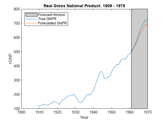
yF is a 10-by-1 vector of future values of real GNP corresponding to the future predictor data.
Estimate the forecast root mean squared error (RMSE).
frmse = sqrt(mean((yF - yFT).^2))
frmse =
25.5397
The forecast RMSE is a relative measure of forecast accuracy. Specifically, you estimate several models using different assumptions. The model with the lowest forecast RMSE is the best-performing model of the ones being compared.
Consider the regression model in Forecast Responses Using Posterior Predictive Distribution.
Create a normal-inverse-gamma semiconjugate prior model for the linear regression parameters. Specify the number of predictors p and the names of the regression coefficients.
p = 3;
PriorMdl = bayeslm(p,'ModelType','semiconjugate','VarNames',["IPI" "E" "WR"]);
Load the Nelson-Plosser data set. Create variables for the response and predictor series.
load Data_NelsonPlosser
X = DataTable{:,PriorMdl.VarNames(2:end)};
y = DataTable{:,'GNPR'};
Hold out the last 10 periods of data from estimation so you can use them to forecast real GNP. Turn off the estimation display.
fhs = 10; % Forecast horizon size
X = DataTable{1:(end - fhs),PriorMdl.VarNames(2:end)};
y = DataTable{1:(end - fhs),'GNPR'};
XF = DataTable{(end - fhs + 1):end,PriorMdl.VarNames(2:end)}; % Future predictor data
yFT = DataTable{(end - fhs + 1):end,'GNPR'};                  % True future responses
Forecast responses by using the posterior predictive distribution and the future predictor data XF. Specify the in-sample observations X and y (the observations from which MATLAB® composes the posterior).
yF = forecast(PriorMdl,XF,X,y)
yF = 10×1

  491.5404
  518.1725
  539.0625
  566.7594
  597.7005
  633.4666
  644.7270
  672.7937
  693.5321
  678.2268
Consider the regression model in Forecast Responses Using Posterior Predictive Distribution.
Assume these prior distributions for = 0,...,3:
, where and are independent, standard normal random variables. Therefore, the coefficients have a Gaussian mixture distribution. Assume all coefficients are conditionally independent, a priori, but they are dependent on the disturbance variance.
. and are the shape and scale, respectively, of an inverse gamma distribution.
and it represents the random variable-inclusion regime variable with a discrete uniform distribution.
Perform stochastic search variable selection (SSVS):
Create a Bayesian regression model for SSVS with a conjugate prior for the data likelihood. Use the default settings.
Hold out the last 10 periods of data from estimation.
Estimate the marginal posterior distributions.
p = 3;
PriorMdl = bayeslm(p,'ModelType','mixconjugate','VarNames',["IPI" "E" "WR"]);

load Data_NelsonPlosser
fhs = 10; % Forecast horizon size
X = DataTable{1:(end - fhs),PriorMdl.VarNames(2:end)};
y = DataTable{1:(end - fhs),'GNPR'};
XF = DataTable{(end - fhs + 1):end,PriorMdl.VarNames(2:end)}; % Future predictor data
yFT = DataTable{(end - fhs + 1):end,'GNPR'};                  % True future responses

rng(1); % For reproducibility
PosteriorMdl = estimate(PriorMdl,X,y,'Display',false);
Forecast responses using the posterior predictive distribution and the future predictor data XF. Plot the true values of the response and the forecasted values.
yF = forecast(PosteriorMdl,XF);

figure;
plot(dates,DataTable.GNPR);
hold on
plot(dates((end - fhs + 1):end),yF)
h = gca;
hp = patch([dates(end - fhs + 1) dates(end) dates(end) dates(end - fhs + 1)],...
    h.YLim([1,1,2,2]),[0.8 0.8 0.8]);
uistack(hp,'bottom');
legend('Forecast Horizon','True GNPR','Forecasted GNPR','Location','NW')
title('Real Gross National Product: 1909 - 1970');
ylabel('rGNP');
xlabel('Year');
hold off
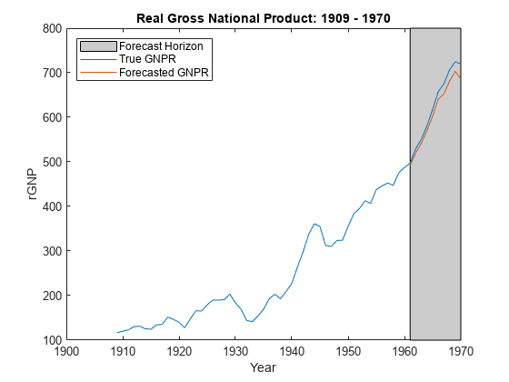
yF is a 10-by-1 vector of future values of real GNP corresponding to the future predictor data.
Estimate the forecast root mean squared error (RMSE).
frmse = sqrt(mean((yF - yFT).^2))
frmse =
18.8470
The forecast RMSE is a relative measure of forecast accuracy. Specifically, you estimate several models using different assumptions. The model with the lowest forecast RMSE is the best-performing model of the ones being compared.
When you perform Bayesian regression with SSVS, a best practice is to tune the hyperparameters. One way to do so is to estimate the forecast RMSE over a grid of hyperparameter values, and choose the value that minimizes the forecast RMSE.
Consider the regression model in Forecast Responses Using Posterior Predictive Distribution.
Create a normal-inverse-gamma semiconjugate prior model for the linear regression parameters. Specify the number of predictors p and the names of the regression coefficients.
p = 3;
PriorMdl = bayeslm(p,'ModelType','semiconjugate','VarNames',["IPI" "E" "WR"]);
Load the Nelson-Plosser data set. Create variables for the response and predictor series.
load Data_NelsonPlosser
X = DataTable{:,PriorMdl.VarNames(2:end)};
y = DataTable{:,'GNPR'};
Hold out the last 10 periods of data from estimation so you can use them to forecast real GNP. Turn off the estimation display.
fhs = 10; % Forecast horizon size
X = DataTable{1:(end - fhs),PriorMdl.VarNames(2:end)};
y = DataTable{1:(end - fhs),'GNPR'};
XF = DataTable{(end - fhs + 1):end,PriorMdl.VarNames(2:end)}; % Future predictor data
yFT = DataTable{(end - fhs + 1):end,'GNPR'};                  % True future responses
Forecast responses by using the conditional posterior predictive distribution of beta given and using the future predictor data XF. Specify the in-sample observations X and y (the observations from which MATLAB® composes the posterior). Plot the true values of the response and the forecasted values.
yF = forecast(PriorMdl,XF,X,y,'Sigma2',2);

figure;
plot(dates,DataTable.GNPR);
hold on
plot(dates((end - fhs + 1):end),yF)
h = gca;
hp = patch([dates(end - fhs + 1) dates(end) dates(end) dates(end - fhs + 1)],...
    h.YLim([1,1,2,2]),[0.8 0.8 0.8])
hp =
  Patch with properties:

    FaceColor: [0.8000 0.8000 0.8000]
    FaceAlpha: 1
    EdgeColor: [0.1294 0.1294 0.1294]
    LineStyle: '-'
        Faces: [1 2 3 4]
     Vertices: [4×2 double]

  Show all properties
uistack(hp,'bottom');
legend('Forecast Horizon','True GNPR','Forecasted GNPR','Location','NW')
title('Real Gross National Product: 1909 - 1970');
ylabel('rGNP');
xlabel('Year');
hold off

Consider the regression model in Forecast Responses Using Posterior Predictive Distribution.
Create a normal-inverse-gamma semiconjugate prior model for the linear regression parameters. Specify the number of predictors p and the names of the regression coefficients.
p = 3;
PriorMdl = bayeslm(p,'ModelType','semiconjugate','VarNames',["IPI" "E" "WR"]);
Load the Nelson-Plosser data set. Create variables for the response and predictor series.
load Data_NelsonPlosser
X = DataTable{:,PriorMdl.VarNames(2:end)};
y = DataTable{:,'GNPR'};
Hold out the last 10 periods of data from estimation so you can use them to forecast real GNP. Turn off the estimation display.
fhs = 10; % Forecast horizon size
X = DataTable{1:(end - fhs),PriorMdl.VarNames(2:end)};
y = DataTable{1:(end - fhs),'GNPR'};
XF = DataTable{(end - fhs + 1):end,PriorMdl.VarNames(2:end)}; % Future predictor data
yFT = DataTable{(end - fhs + 1):end,'GNPR'};                  % True future responses
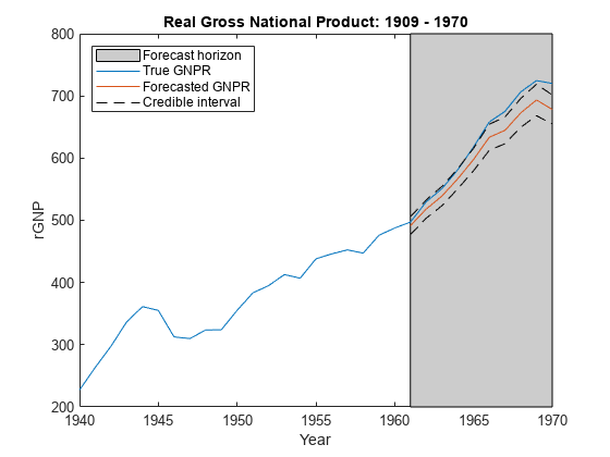
Forecast responses and their covariance matrix by using the posterior predictive distribution and the future predictor data XF. Specify the in-sample observations X and y (the observations from which MATLAB® composes the posterior).
[yF,YFCov] = forecast(PriorMdl,XF,X,y);
Because the predictive posterior distribution is not analytical, a reasonable approximation to a set of 95% credible intervals is
for all in the forecast horizon. Estimate 95% credible intervals for the forecasts using this formula.
n = sum(all(~isnan([X y]')));
cil = yF - norminv(0.975)*sqrt(diag(YFCov));
ciu = yF + norminv(0.975)*sqrt(diag(YFCov));
Plot the data, forecasts, and forecast intervals.
figure;
plot(dates(end-30:end),DataTable.GNPR(end-30:end));
hold on
h = gca;
plot(dates((end - fhs + 1):end),yF)
plot(dates((end - fhs + 1):end),[cil ciu],'k--')
hp = patch([dates(end - fhs + 1) dates(end) dates(end) dates(end - fhs + 1)],...
    h.YLim([1,1,2,2]),[0.8 0.8 0.8]);
uistack(hp,'bottom');
legend('Forecast horizon','True GNPR','Forecasted GNPR',...
    'Credible interval','Location','NW')
title('Real Gross National Product: 1909 - 1970');
ylabel('rGNP');
xlabel('Year');
hold off
Input Arguments
Name-Value Arguments
Output Arguments
Limitations
If Mdl is an empiricalblm model object, then you cannot specify
Beta or Sigma2. You cannot forecast from
conditional predictive distributions by using an empirical prior distribution.
More About
Tips
Monte Carlo simulation is subject to variation. If
forecastuses Monte Carlo simulation, then estimates and inferences might vary when you callforecastmultiple times under seemingly equivalent conditions. To reproduce estimation results, set a random number seed by usingrngbefore callingforecast.If
forecastissues an error while estimating the posterior distribution using a custom prior model, then try adjusting initial parameter values by usingBetaStartorSigma2Start, or try adjusting the declared log prior function, and then reconstructing the model. The error might indicate that the log of the prior distribution is–Infat the specified initial values.To forecasted responses from the conditional posterior predictive distribution of analytically intractable models, except empirical models, pass your prior model object and the estimation-sample data to
forecast. Then, specify theBetaname-value pair argument to forecast from the conditional posterior of σ2, or specify theSigma2name-value pair argument to forecast from the conditional posterior of β.
Algorithms
Whenever
forecastmust estimate a posterior distribution (for example, whenMdlrepresents a prior distribution and you supplyXandy) and the posterior is analytically tractable,forecastevaluates the closed-form solutions to Bayes estimators. Otherwise,forecastresorts to Monte Carlo simulation to forecast by using the posterior predictive distribution. For more details, see Posterior Estimation and Inference.This figure illustrates how
forecastreduces the Monte Carlo sample using the values ofNumDraws,Thin, andBurnIn. Rectangles represent successive draws from the distribution.forecastremoves the white rectangles from the Monte Carlo sample. The remainingNumDrawsblack rectangles compose the Monte Carlo sample.
Version History
Introduced in R2017a
See Also
Objects
conjugateblm|semiconjugateblm|diffuseblm|empiricalblm|customblm|mixconjugateblm|mixsemiconjugateblm|lassoblm