Audio Transfer Learning Using Experiment Manager

This example shows how to configure an experiment that compares the performance of multiple pretrained networks in a speech command recognition task using transfer learning. This example uses the Experiment Manager app to tune hyperparameters and compare results between the different pretrained networks by using both built-in and user-defined metrics.

Audio Toolbox™ provides a variety of pretrained networks for audio processing, and each network has a different architecture that requires different data preprocessing. These differences result in tradeoffs between the accuracy, speed, and size of the various networks. Experiment Manager organizes the results of the training experiments to highlight the strengths and weaknesses of each individual network so you can select the network that best fits your constraints.

The example compares the performance of the YAMNet (Audio Toolbox) and VGGish (Audio Toolbox) pretrained networks, as well as a custom network that you train from scratch. See Deep Network Designer to explore other pretrained network options supported by Audio Toolbox™.

This example uses the Google Speech Commands [1] data set. Download the data set and the pretrained networks to your temporary directory. The data set and the two networks require 1.96 GB and 470 MB of disk space, respectively.

Open Experiment Manager

Load the example by clicking the Open Example button. This opens the project in Experiment Manager in your MATLAB editor.

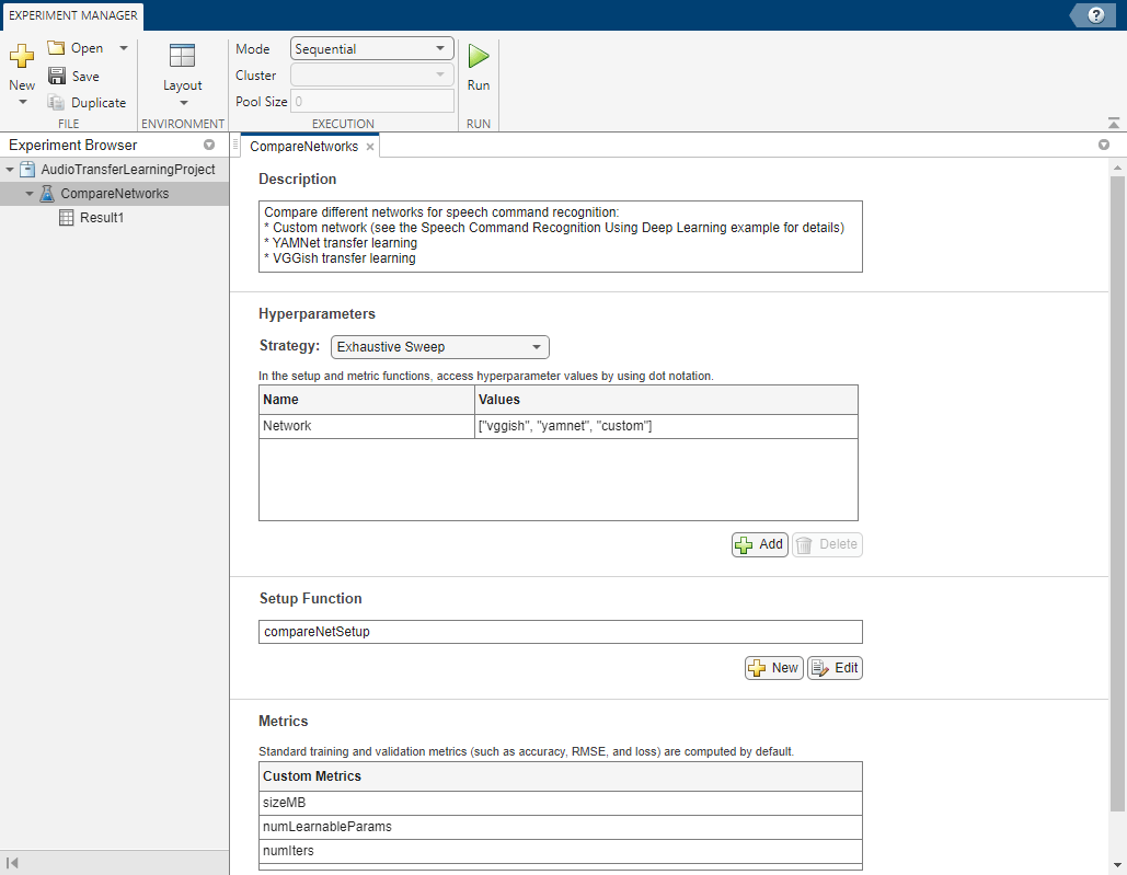
Built-in training experiments consist of a description, a table of hyperparameters, a setup function, and a collection of metric functions to evaluate the results of the experiment. For more information, see Train Network Using trainnet and Display Custom Metrics.

The Description field contains a description of the experiment.

The Hyperparameters section specifies the strategy and hyperparameter values to use for the experiment. This example uses the exhaustive sweep strategy. When you run the experiment, Experiment Manager trains the network using every combination of the hyperparameter values specified in the hyperparameter table. As this example shows you how to test the different network types, define one hyperparameter, Network, to represent the network names stored as strings.

The Setup Function field contains the name of the main function that configures the training data, network architecture, and training options for the experiment. The input to the setup function is a structure with fields from the hyperparameter table. The setup function returns the training data, network architecture, and training parameters as outputs. This example uses a predesigned setup function named compareNetSetup.

The Metrics list enables you to define your own custom metrics to compare across different trials of the training experiment. Experiment Manager runs each of metric in this table against the networks it trains in each trial. This example defines three custom metrics. To add additional custom metrics, list them in this table.

Define Setup Function

In this example, the setup function downloads the data set, selects the desired network, performs the requisite data preprocessing, and sets the network training options. The input to this function is a structure with fields for each hyperparameter you define in the Experiment Manager interface. In the setup function for this example, the input variable is params and the output variables are trainingData, layers, and options, representing the training data, network structure, and training parameters, respectively. The key steps of the compareNetSetup setup function are explained below. Open the example in MATLAB to see the full definition of the function.

Download and Extract Data

To speed up the example, open compareNetSetup and set the speedUp flag to true. This reduces the size of the data set to quickly test the basic functionality of the experiment.

speedUp = true;

The helper function setupDatastores downloads the Google Speech Commands [1] data set, selects the commands for networks to recognize, and randomly partitions the data into training and validation datastores.

[adsTrain,adsValidation] = setupDatastores(speedUp);

Select Network and Preprocess Data

Transform the datastores based on the preprocessing required by each network you define in the hyperparameter table, which you can access using params.Network. The helper function extractSpectrogram processes the input data to the format required by each network. The helper function getLayers returns a layerGraph object that represents the architecture of the network.

tdsTrain = transform(adsTrain,@(x)extractSpectrogram(x,params.Network));
tdsValidation = transform(adsValidation,@(x)extractSpectrogram(x,params.Network));

layers = getLayers(classes,classWeights,numClasses,netName);

Now that you have set up the datastores, read the data into the trainingData and validationData variables.

trainingData = readall(tdsTrain,UseParallel=canUseParallelPool);
validationData = readall(tdsValidation,UseParallel=canUseParallelPool);

validationData = table(validationData(:,1),adsValidation.Labels);
trainingData = table(trainingData(:,1),adsTrain.Labels);

Set the Training Options

Set the training parameters by assigning a trainingOptions object to the options output variable. Train the networks for a maximum of 30 epochs with a patience of 8 epochs using the Adam optimizer. Set the ExecutionEnvironment field to "auto" to use a GPU if available. Training can be time consuming if you do not use a GPU.

maxEpochs = 30;
miniBatchSize = 256;
validationFrequency = floor(numel(TTrain)/miniBatchSize);
options = trainingOptions("adam", ...
    GradientDecayFactor=0.7, ...
    InitialLearnRate=params.LearnRate, ...
    MaxEpochs=maxEpochs, ...
    MiniBatchSize=miniBatchSize, ...
    Shuffle="every-epoch", ...
    Plots="training-progress", ...
    Verbose=false, ...
    ValidationData=validationData, ...
    ValidationFrequency=validationFrequency, ...
    ValidationPatience=10, ...
    LearnRateSchedule="piecewise", ...
    LearnRateDropFactor=0.2, ...
    LearnRateDropPeriod=round(maxEpochs/3), ...
    ExecutionEnvironment="auto");

Define Custom Metrics

Experiment Manager enables you to define custom metric functions to evaluate the performance of the networks it trains in each trial. It computes basic metrics such as accuracy and loss by default. In this example you compare the size of each of the models as memory usage is an important metric when you deploy deep neural networks to real-world applications.

Custom metric functions must take one input argument trialInfo, which is a structure containing the fields trainedNetwork, trainingInfo, and parameters.

• trainedNetwork is the SeriesNetwork object or DAGNetwork object returned by the trainNetwork function.

• trainingInfo is a structure containing the training information returned by the trainNetwork function.

• parameters is a struct with fields from the hyperparameter table

The metric functions must return a scalar number, logical output, or string which the Experiment Manager displays in the results table. The example uses these custom metric functions:

• sizeMB computes the memory allocated to store the networks in megabytes

• numLearnableParams counts the number of learnable parameters within each model

• numIters computes the number of mini-batches used to train each network before reaching the MaxEpochs parameter or violating the ValidationPatience parameter in the trainingOptions object.

Run Experiment

Click Run on the Experiment Manager toolstrip to run the experiment. You can select to run each trial sequentially, simultaneously, or in batches by using the mode option. For this experiment, set Mode to Sequential.

Evaluate Results

Experiment Manager displays the results in a table once it finishes running the experiment. The progress bar shows how many epochs each network trained for before violating the patience parameter in terms of the percentage of MaxEpochs.

You can sort the table by each column by pointing to the column name and clicking the arrow that appears. Click the table icon on the top right corner to select which columns to show or hide. To first compare the networks by accuracy, sort the table over the Validation Accuracy column in descending order.

In terms of accuracy, the Yamnet network performs the best followed by VGGish networi, and then the custom network. However, sorting by the Elapsed Time column shows that Yamnet takes the longest to train. To compare the size of these networks, sort the table by the sizeMB column.

The custom network is the smallest, Yamnet is a few orders of magnitude larger, and VGGish is the largest.

These results highlight the tradeoffs between the different network designs. The Yamnet network performs the best at the classification task at the cost of more training time and moderately large memory consumption. The VGGish network performs slightly worse in terms of accuracy and requires over 20 times more memory than YAMNet. Lastly, the custom network has the worst accuracy by a small margin, but the network also uses the least memory.

Even though Yamnet and VGGish are pretrained networks, the custom network converges the fastest. Looking at the NumIters column, the custom network takes the most batch iterations to converge because it is learning from scratch. As the custom network is much smaller and shallower than the deep pretrained models, each of these batch updates are processed much faster, thereby reducing the overall training time.

To save one of the trained networks from any of the trials, right-click the corresponding row in the results table and select Export Trained Network.

To further analyze a trial, click on the corresponding row, and under the Review Results tab in the app toolstrip, choose to plot of the training progress or a confusion matrix of the trained model. This diagram shows the confusion matrix for the Yamnet model from trial 2 of the experiment.

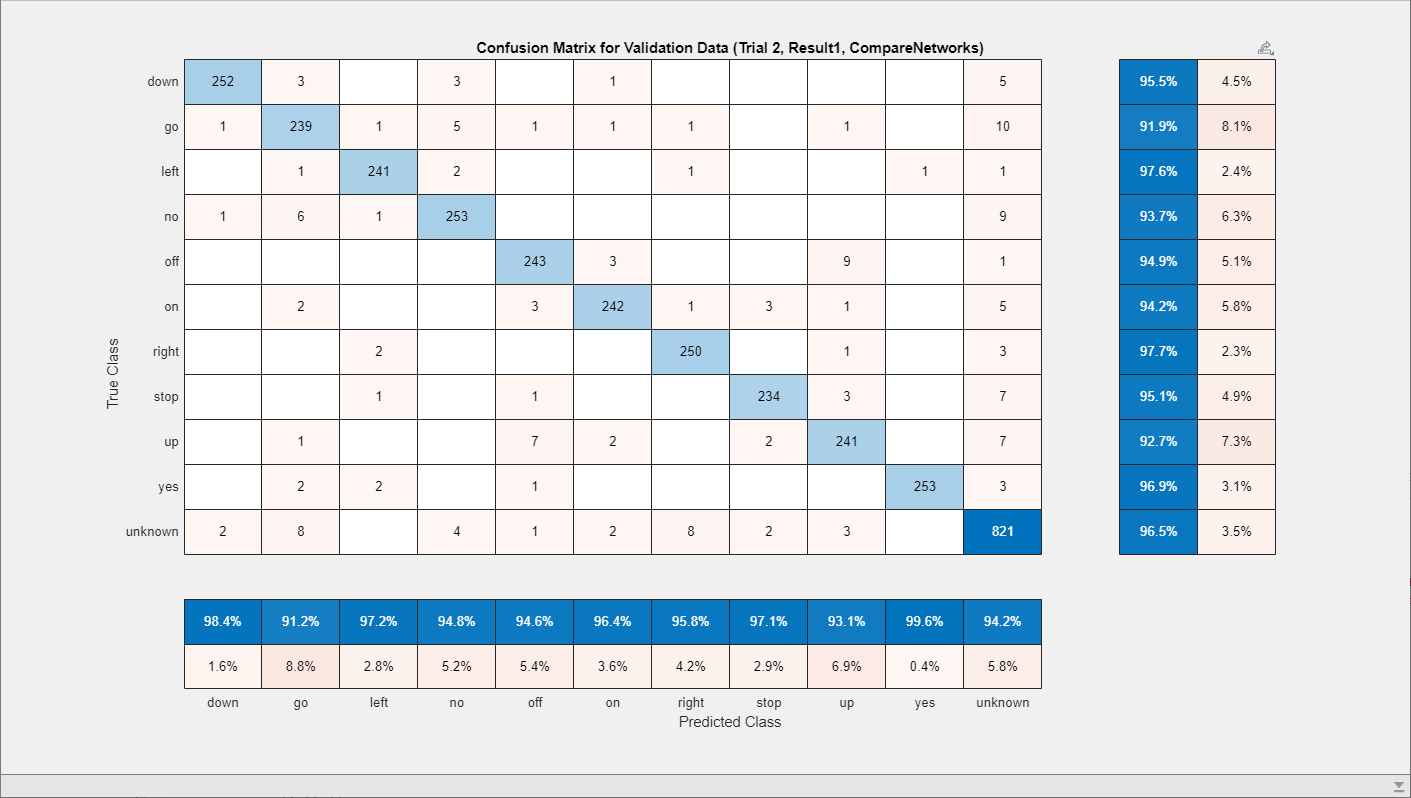
The model struggles most at differentiating between the "off" and "up" and "no" and "go" commands, although the accuracy is generally uniform across all classes. Further, the model successfully predicts the "yes" command as the false positive rate for that class is only 0.4%.

References

[1] Warden P. "Speech Commands: A public dataset for single-word speech recognition", 2017. Available from https://storage.googleapis.com/download.tensorflow.org/data/speech_commands_v0.01.tar.gz. Copyright Google 2017. The Speech Commands Dataset is licensed under the Creative Commons Attribution 4.0 license, available here: https://creativecommons.org/licenses/by/4.0/legalcode.