Acoustics-Based Machine Fault Recognition Code Generation with Intel MKL-DNN

This example uses:

This example demonstrates code generation for Acoustics-Based Machine Fault Recognition (Audio Toolbox) using a long short-term memory (LSTM) network and spectral descriptors. This example uses MATLAB® Coder™ with deep learning support to generate a MEX (MATLAB executable) function that leverages performance of Intel® MKL-DNN library. The input data consists of acoustics time-series recordings from faulty or healthy air compressors and the output is the state of the mechanical machine predicted by the LSTM network. For details on audio preprocessing and network training, see Acoustics-Based Machine Fault Recognition (Audio Toolbox).

Example Requirements

The MATLAB Coder Interface for Deep Learning Support Package
Intel processor with support for Intel Advanced Vector Extensions 2 (Intel AVX2)
Intel Deep Neural Networks Library (MKL-DNN)
Environment variables for Intel MKL-DNN

For supported versions of libraries and for information about setting up environment variables, see Prerequisites for Deep Learning with MATLAB Coder (MATLAB Coder).

Prepare Input Dataset

Specify a sample rate fs of 16 kHz and a windowLength of 512 samples, as defined in Acoustics-Based Machine Fault Recognition (Audio Toolbox). Set numFrames to 100.

fs = 16000;
windowLength = 512;
numFrames = 100;

To run the Example on a test signal, generate a pink noise signal. To test the performance of the system on a real dataset, download the air compressor dataset [1].

downloadDataset = false;

if ~downloadDataset
    pinkNoiseSignal = pinknoise(windowLength*numFrames);
else
    % Download AirCompressorDataset.zip 
    component = 'audio';
    filename = 'AirCompressorDataset/AirCompressorDataset.zip';
    localfile = matlab.internal.examples.downloadSupportFile(component,filename);
    
    % Unzip the downloaded zip file to the downloadFolder
    downloadFolder = fileparts(localfile);
    if ~exist(fullfile(downloadFolder,'AirCompressorDataset'),'dir')
        unzip(localfile, downloadFolder)
    end
    
    % Create an audioDatastore object dataStore, to manage, the data.
    dataStore = audioDatastore(downloadFolder,'IncludeSubfolders',true,'LabelSource','foldernames');

    % Use countEachLabel to get the number of samples of each category in the dataset.
    countEachLabel(dataStore)
end

Recognize Machine Fault in MATLAB

To run the streaming classifier in MATLAB, download and unzip the system developed in Acoustics-Based Machine Fault Recognition (Audio Toolbox).

component = 'audio';
filename = 'AcousticsBasedMachineFaultRecognition/AcousticsBasedMachineFaultRecognition.zip';
localfile = matlab.internal.examples.downloadSupportFile(component,filename);

downloadFolder = fullfile(fileparts(localfile),'system');
if ~exist(downloadFolder,'dir')    
    unzip(localfile,downloadFolder)
end

To access the recognizeAirCompressorFault function of the system, add downloadFolder to the search path.

addpath(downloadFolder)

Create a dsp.AsyncBuffer (DSP System Toolbox) object to read audio in a streaming fashion and a dsp.AsyncBuffer (DSP System Toolbox) object to accumulate scores.

audioSource = dsp.AsyncBuffer;
scoreBuffer = dsp.AsyncBuffer;

Load the pretrained network and extract labels from the network.

airCompNet = coder.loadDeepLearningNetwork('AirCompressorFaultRecognitionModel.mat');
labels = string(airCompNet.Layers(end).Classes);

Initialize signalToBeTested to pinkNoiseSignal or select a signal from the drop-down list to test the file of your choice from the dataset.

if ~downloadDataset
    signalToBeTested = pinkNoiseSignal;
else
    [allFiles,~] = splitEachLabel(dataStore,1);
    allData = readall(allFiles);
    signalToBeTested = allData(6);
    signalToBeTested = cell2mat(signalToBeTested);
end

Stream one audio frame at a time to represent the system as it would be deployed in a real-time embedded system. Use recognizeAirCompressorFault developed in Acoustics-Based Machine Fault Recognition (Audio Toolbox) to compute audio features and perform deep learning classification.

write(audioSource,signalToBeTested);
resetNetworkState = true;

while audioSource.NumUnreadSamples >= windowLength

    % Get a frame of audio data
    x = read(audioSource,windowLength);

    % Apply streaming classifier function
    score = recognizeAirCompressorFault(x,resetNetworkState);
    
    % Store score for analysis
    write(scoreBuffer,score);
    
    resetNetworkState = false;
end

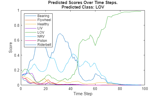
Compute the recognized fault from scores and display it.

scores = read(scoreBuffer);
[~,labelIndex] = max(scores(end,:),[],2);
detectedFault = labels(labelIndex)

detectedFault = 
"Flywheel"

Plot the scores of each label for each frame.

plot(scores)
legend("" + labels,'Location','northwest') 
xlabel("Time Step")
ylabel("Score")
str = sprintf("Predicted Scores Over Time Steps.\nPredicted Class: %s",detectedFault);
title(str)

Generate MATLAB Executable

Create a code generation configuration object to generate an executable. Specify the target language as C++.

cfg = coder.config('mex');
cfg.TargetLang = 'C++';

Create a configuration object for deep learning code generation with the MKL-DNN library. Attach the deep learning configuration object to the code generation configuration object.

dlcfg = coder.DeepLearningConfig('mkldnn');
cfg.DeepLearningConfig = dlcfg;

Create an audio data frame of length windowLength.

audioFrame = ones(windowLength,1);

Call the codegen (MATLAB Coder) function from MATLAB Coder to generate C++ code for the recognizeAirCompressorFault function. Specify the configuration object and prototype arguments. A MEX-file named recognizeAirCompressorFault_mex is generated to your current folder.

codegen -config cfg recognizeAirCompressorFault -args {audioFrame,resetNetworkState} -report

Code generation successful: View report

Perform Machine Fault Recognition Using MATLAB Executable

Initialize signalToBeTested to pinkNoiseSignal or select a signal from the drop-down list to test the file of your choice from the dataset.

if ~downloadDataset
    signalToBeTested = pinkNoiseSignal;
else
    [allFiles,~] = splitEachLabel(dataStore,1);
    allData = readall(allFiles);
    signalToBeTested = allData(8);
    signalToBeTested = cell2mat(signalToBeTested);
end

Stream one audio frame at a time to represent the system as it would be deployed in a real-time embedded system. Use generated recognizeAirCompressorFault_mex to compute audio features and perform deep learning classification.

write(audioSource,signalToBeTested);
resetNetworkState = true;

while audioSource.NumUnreadSamples >= windowLength

    % Get a frame of audio data
    x = read(audioSource,windowLength);

    % Apply streaming classifier function
    score = recognizeAirCompressorFault_mex(x,resetNetworkState);
    
    % Store score for analysis
    write(scoreBuffer,score);

    resetNetworkState = false;
end

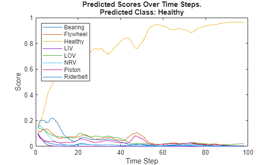
Compute the recognized fault from scores and display it.

scores = read(scoreBuffer);
[~,labelIndex] = max(scores(end,:),[],2);
detectedFault = labels(labelIndex)

detectedFault = 
"Flywheel"

Plot the scores of each label for each frame.

plot(scores)
legend("" + labels,'Location','northwest')
xlabel("Time Step")
ylabel("Score")
str = sprintf("Predicted Scores Over Time Steps.\nPredicted Class: %s",detectedFault);
title(str)

Evaluate Execution Time of Alternative MEX Function Workflow

Use tic and toc to measure the execution time of MATLAB function recognizeAirCompressorFault and MATLAB executable (MEX) recognizeAirCompressorFault_mex.

Create a dsp.AsyncBuffer (DSP System Toolbox) object to record execution time.

timingBufferMATLAB = dsp.AsyncBuffer;
timingBufferMEX = dsp.AsyncBuffer;

Use same recording that you chose in previous section as input to recognizeAirCompressorFault function and its MEX equivalent recognizeAirCompressorFault_mex.

write(audioSource,signalToBeTested);

Measure the execution time of the MATLAB code.

resetNetworkState = true;
while audioSource.NumUnreadSamples >= windowLength

    % Get a frame of audio data
    x = read(audioSource,windowLength);

    % Apply streaming classifier function
    tic
    scoreMATLAB = recognizeAirCompressorFault(x,resetNetworkState);
    write(timingBufferMATLAB,toc);

    % Apply streaming classifier MEX function
    tic
    scoreMEX = recognizeAirCompressorFault_mex(x,resetNetworkState);
    write(timingBufferMEX,toc);

    resetNetworkState = false;

end

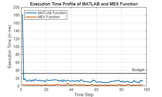
Plot the execution time for each frame and analyze the profile. The first call of recognizeAirCompressorFault_mex consumes around four times of the budget as it includes loading of network and resetting of the states. However, in a real, deployed system, that initialization time is only incurred once. The execution time of the MATLAB function is around 10 ms and that of MEX function is ~1 ms, which is well below the 32 ms budget for real-time performance.

budget = (windowLength/fs)*1000;
timingMATLAB = read(timingBufferMATLAB)*1000;
timingMEX = read(timingBufferMEX)*1000;
frameNumber = 1:numel(timingMATLAB);
perfGain = timingMATLAB./timingMEX;
plot(frameNumber,timingMATLAB,frameNumber,timingMEX,'LineWidth',2)
grid on
yline(budget,'',{'Budget'},'LineWidth',2)
legend('MATLAB Function','MEX Function','Location','northwest')
xlabel("Time Step")
ylabel("Execution Time (in ms)")
title("Execution Time Profile of MATLAB and MEX Function")

Compute the performance gain of MEX over MATLAB function excluding the first call. This performance test is done on a machine using an NVIDIA Quadro P620 (Version 26) GPU and an Intel® Xeon® W-2133 CPU running at 3.60 GHz.

PerformanceGain = sum(timingMATLAB(2:end))/sum(timingMEX(2:end))

PerformanceGain = 24.0484

This example ends here. For deploying machine fault recognition on Raspberry Pi, see Acoustics-Based Machine Fault Recognition Code Generation on Raspberry Pi (Audio Toolbox).

References

[1] Verma, Nishchal K., et al. "Intelligent Condition Based Monitoring Using Acoustic Signals for Air Compressors." IEEE Transactions on Reliability, vol. 65, no. 1, Mar. 2016, pp. 291–309. DOI.org (Crossref), doi:10.1109/TR.2015.2459684.