Main Content

splinetool

Experiment with some spline approximation methods

Description

splinetool opens the Spline Tool, which lets you experiment with various spline approximation methods. It provides you with choices for data, including the option of importing some data from the workspace.

splinetool(x,y)opens the tool with the specified data x and y, which must be vectors of the same length.

example

Examples

collapse all

Run this code to open the Spline Tool and experiment with noisy data.

x = linspace(1,pi,101); 
y = cos(x)+(rand(size(x))-.5)/10;
splinetool(x,y)

This example shows how to explore the various end conditions available with cubic spline interpolation in the Spline Tool.

  1. Type splinetool at the command line.

  2. Select Import your own data from the initial screen, and accept the default function. You should see the following display.

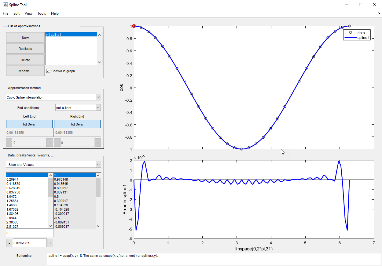
    Spline Tool showing the cubic spline interpolant approximation with the not-a-knot end condition

    The default approximation is the cubic spline interpolant with the not-a-knot end condition.

    The vector x of data sites is linspace(0,2*pi,31) and the values are cos(x). This differs from simply providing the vector y of values in that the cosine function is explicitly recorded as the underlying function. Therefore, the error shown in the graph is the error in the spline as an approximation to the cosine rather than as an approximation to the given values. Notice the resulting relatively large error, about 5e-5, near the endpoints.

  3. For comparison, follow these steps:

    1. Click New in the List of approximations.

    2. In Approximation method, select complete from the list of End conditions.

    3. Since the first derivative of the cosine function is sine, adjust the first-derivative values to their known values of zero at both the left end and the right end.

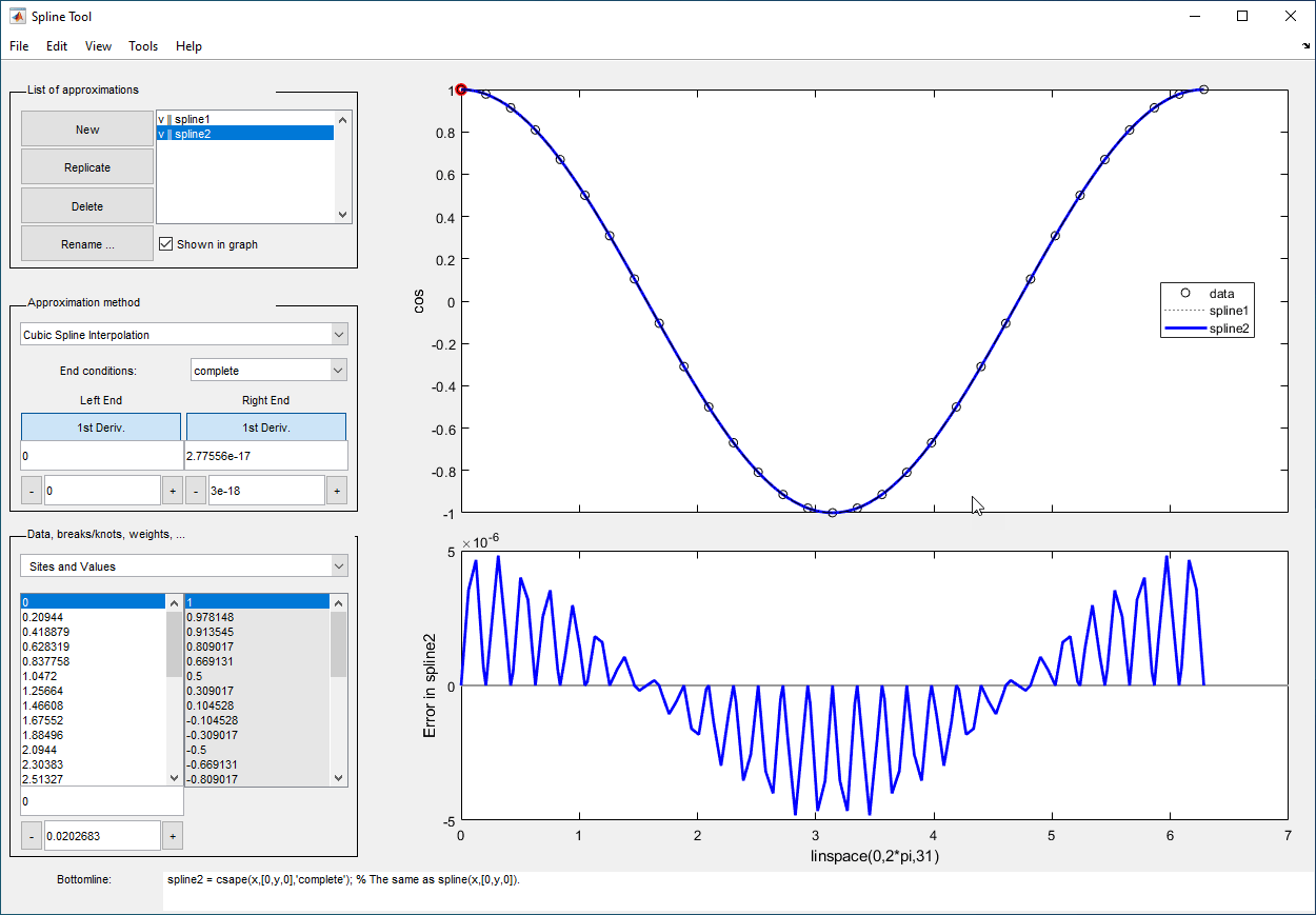
    This procedure results in the display shown below. The right end slope is zero only up to round-off. Bottomline tells you that the tool uses the function csape to create the spline.

    Spline tool showing a comparison of cubic spline interpolant approximation with the not-a-knot end condition and the complete end condition.

    The improvement in the error is only about 5e-6.

  4. For further comparison, follow these steps:

    1. Click New in the List of approximations.

    2. In Approximation method, select natural from the list of End conditions.

    Note the deterioration of the approximation near the ends, an error of about 2e-3, which is much worse than with the not-a-knot end conditions.

  5. For a final comparison, follow these steps:

    1. Click New in the List of approximations.

    2. Since the cosine function is periodic, in Approximation method, select periodic from the list of End conditions.

    Note the dramatic improvement in the approximation, back to an error of about 5e-6, particularly compared to the natural end conditions.

This example uses cubic spline interpolation and least-squares approximation in the Spline Tool to determine an estimate of the initial acceleration for a drag car.

  1. Type splinetool at the command line or if the tool is already open, click File > Restart.

  2. Select Richard Tapia's drag race data. The data shows the distance traveled by a drag car as a function of time. The message window asks you to estimate the initial acceleration by setting the initial speed to zero. Click OK, or press the space bar or Enter, to remove the message window.

  3. In Approximation method, select complete from the list of End conditions.

  4. Adjust the initial speed by changing the first derivative at the left endpoint to zero.

  5. Look for the value of the initial acceleration, which is given by the value of the second derivative at the left endpoint. You can toggle between the first derivative and the second derivative at this endpoint by clicking on the left end button. The value of the second derivative should be around 187 in the units chosen. Select View > Show 2nd Derivative to see the result graphically.

  6. For comparison, click New, then select Least-Squares Approximation as the Approximation method. With this method, you can no longer specify end conditions. Instead, you may vary the order of the method. Verify that the initial acceleration is close to the cubic interpolation value.

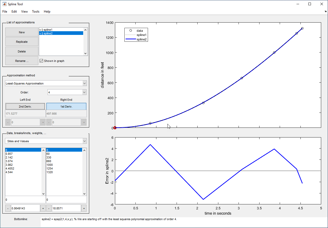
    The results of this procedure are shown below.

    Spline Tool showing least-squares approximation of order 4 for Richard Tapia's drag race data

This example encourages you to place five interior knots in such a way that the least-squares approximation by cubic splines has an absolute error no bigger than .04 everywhere.

  1. Type splinetool at the command line or if the tool is already open, click File > Restart.

  2. Select Titanium heat data.

  3. Select Least-Squares Approximation as the Approximation method.

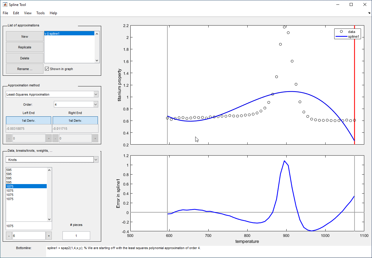
  4. Notice how poorly this selection approximates the data since there are no interior knots. To view the current knots and add new knots, select Knots from Data, breaks/knots, weights. The knots are now listed in Knots, and also displayed in the data graph as vertical lines. There are just the two end knots, each with multiplicity 4.

  5. Right-click in the data graph and select Add Knot. This option displays a crosshairs for you to move with the mouse. Its precise horizontal location is shown in the edit field below the list of knots. A mouse click places a new knot at the current location of the crosshairs. One possible strategy is to add the knot at the place of maximum absolute error, as shown in the auxiliary graph below the data graph.

    Spline Tool showing the least square approximation for titanium heat data and the two end knots

    If you right-click and select Replicate Knot, you increase the multiplicity of the current knot, which is reflected by its repeated occurrence in Knots. To delete a specific knot, first select it in either the list of knots or the data graph, and then right-click in the graph and select Delete Knot.

  6. You can also opt for an approximation using six polynomial pieces, which corresponds to five interior knots. To specify this option, enter 6 as # pieces in Data, breaks/knots, weights.

  7. After you have the five interior knots, try to make the error even smaller by moving the knots. To select the knot you want to move, click its vertical line in the graph, and then use the control below Knots in Data, breaks/knots, weights and observe how the error changes with the movement of the knot. You can also use the edit field to overwrite the current knot location. Also try adjust, which redistributes the current knot sequence.

  8. Use Replicate in List of approximations to save any good knot distribution for later use. Rename the replicated approximation to lstsqr by using Rename. To return to the original approximation, click on its name in List of approximations.

This example experiments with smoothing splines using the Spline Tool.

  1. Type splinetool at the command line or, if the tool is already open, click File > Restart.

  2. Select Titanium heat data.

  3. In Approximation method, select Smoothing Spline.

  4. Vary Parameter between 0 and 1, which changes the approximation from the least-squares straight-line approximation to the “natural” cubic spline interpolant.

  5. Vary Tolerance between 0 and some large value, even inf. The approximation changes from the best possible one, the “natural” cubic spline interpolant, to the least-squares straight-line approximation.

  6. As you increase the Parameter value or decrease the Tolerance value, the error decreases. However, a smaller error corresponds to more roughness, as measured by the size of the second derivative. To see this result, select View > Show 2nd Derivative and vary the Parameter and Tolerance values once again.

  7. Modify the weights in the roughness measure to permit a more accurate but less smooth approximation in the peak area while having a smoother, less accurate, approximation away from the peak area.

    1. Select Jumps in Roughness Weight from Data, breaks/knots, weights.

    2. Select View > Show 2nd Derivative.

    3. Select any data point to the left of the peak in the data.

    4. Set the jump at the selected site to -1 by changing its value in the edit field below it. Since the roughness weight for the very first site interval is 1, you have just set the roughness weight to the right of the highlighted site to 0. Correspondingly, the second derivative has become relatively small to the left of that site.

    5. Select any data point to the right of the peak in the data.

    6. Set the jump across the selected site to 1. Since the roughness weight just to the left of the highlighted site is 0, you have just set the roughness weight to the right of the highlighted site to 1. Correspondingly, the second derivative has become relatively small to the right of that site. The total effect is a very smooth but not very accurate fit away from the peak, while in the peak area, the spline fit is much better but the second derivative is much larger, as is shown in the auxiliary graph below.

      At the sites where there is a jump in the roughness weight, there is a corresponding jump in the second derivative. If you increase the Parameter value, the error across the peak area decreases, but the second derivative remains quite large, while the opposite holds true away from the peak area.

      Spline Tool showing a smoothing spline of order 4 for the titanium heat data

Input Arguments

collapse all

Data sites, specified as a vector of the same length of y. The data sites do not need to be distinct or ordered, but there must be at least two distinct sites.

Data values, specified as a vector of the same length of x.

Tips

Spline Tool is shown in the following figure comparing cubic spline interpolation with a smoothing spline on sample data created by adding noise to the cosine function.
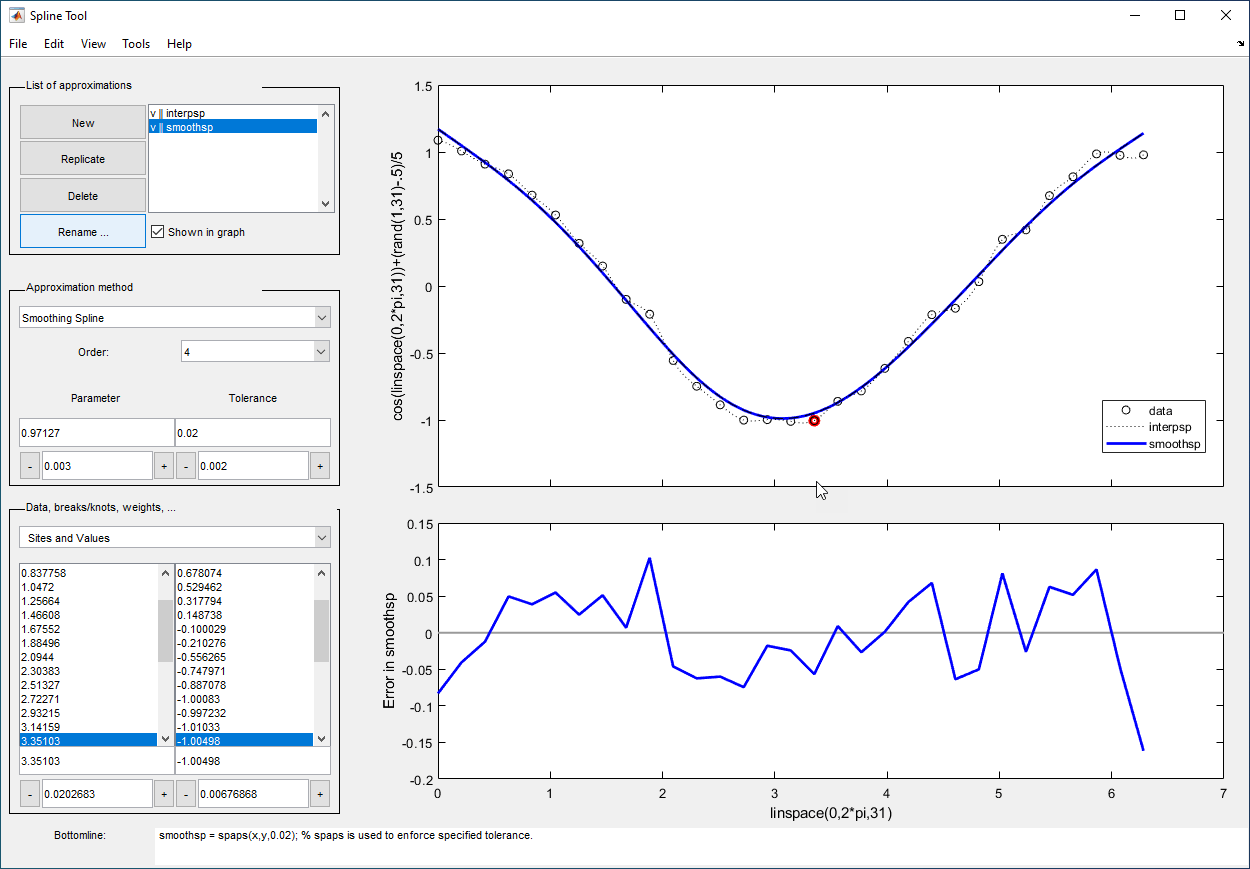
Spline Tool showing a comparison of cubic spline interpolation and a smoothing spline on sample data created by adding noise to the cosine function

Select Approximation Methods

The approximation methods and options supported by the tool are shown below.

Approximation Method

Option

Cubic Interpolating Spline

Adjust the type and values of the end conditions.

Smoothing Spline

Choose between cubic (order 4) and quintic (order 6) splines. Adjust the value of the tolerance and/or smoothing parameter. Adjust the weights in the error and roughness measures.

Least-Squares Approximation

Vary the order from 1 to 14. The default order is 4, which gives cubic approximating splines. Modify the number of polynomial pieces. Add and move knots to improve the fit. Adjust the weights in the error measure.

Spline Interpolation

Vary the order from 2 to 14. The default order is 4, which gives cubic spline interpolants. If the default knots supplied are not satisfactory, you can move them around to vary the fit.

Plot Graphs

You can generate and compare several approximations to the same data. One of the approximations is always marked as “current” using a thicker line width. The following displays are available:

  • Data graph. It shows:

    • Data

    • Approximations chosen for display in List of approximations

    • Current knot sequence or the current break sequence

  • Auxiliary graph (if viewed) for the current approximation. You can view this graph by selecting any one of the items in the View menu. It shows one of the following:

    • First derivative

    • Second derivative

    • Error

By default, the error is the difference between the given data values and the value of the approximation at the data sites. In particular, the error is zero (up to round-off) when the approximation is an interpolant. However, if you provide the data values by specifying a function, then the error displayed is the difference between that function and the current approximation. This also happens if you change the y-label of the data graph to the name of a function.

Try Menu Options

You can annotate and print the graphs with the File > Print to Figure menu.

You can export the data and approximations to the workspace for further use or analysis with the File > Export Data and File > Export Spline menus, respectively.

You can create, with the File > Generate Code menu, a function file that you can use to generate, from the original data, any or all graphs currently shown. This file also provides you with a written record of the commands used to generate the current graphs.

You can save, with the Replicate button, the current approximation before you experiment further. If, at a later time, you click the saved approximation, the tool restores everything to the way it was, including the data used in the construction of the saved approximation. The saved approximation persists even if you have edited the data while working on other approximations.

You can add, delete, or move data, knots, and breaks by right-clicking in the graph, or by selecting the appropriate item in the Edit menu.

You can toggle the grid or the legend in a graph with the Tools menu.

Version History

Introduced before R2006a