Interpolation with Curve Fitting Toolbox
Interpolation is a process for estimating values that lie between known data points.
Interpolation involves creating of a function f that matches given data values yi at given data sites xi where f(xi) = yi, for all i.
Most interpolation methods create the interpolant f as the unique function of the formula
where the form of the functions fj depends on the interpolation method.
For spline interpolation, the fj are the n consecutive B-splines Bj(x) = B(x|tj,...,tj+k), j = 1:n, of order k for a knot sequence t1 ≤ t2 ≤ ... ≤ tn + k.
About Interpolation Methods
Curve Fitting Toolbox™ supports the interpolation methods described in the following table.
Method | Description |
|---|---|
Nearest neighbor | Nearest neighbor interpolation. This method sets the value of an interpolated point to the value of the nearest data point. |
Linear | Linear interpolation. This method fits a different linear polynomial between each pair of data points for curves, or between sets of three points for surfaces. |
Natural neighbor | Natural neighbor interpolation. This method sets the value of an interpolated point to a weighted average of the nearest data points. The interpolating surface is C1 continuous, except at the sample points. |
Shape-preserving (PCHIP) | Piecewise cubic Hermite interpolation (PCHIP). This method preserves monotonicity and the shape of the data (for curves only). |
Cubic spline | Cubic spline interpolation. This method fits a different cubic polynomial between each pair of data points for curves, or between sets of three points for surfaces. |
Biharmonic (v4) | MATLAB® 4 |
Thin-plate spline | Thin-plate spline interpolation. This method fits smooth surfaces that also extrapolate well (for surfaces only). |
Interpolant surface fits use the MATLAB function scatteredInterpolant for the linear,
nearest neighbor, and natural neighbor methods, and the MATLAB function griddata for the cubic spline and
biharmonic methods. The thin-plate spline method uses the tpaps function.
The interpolant method you use depends on several factors, including the characteristics of the data being fit, the required smoothness of the curve, speed considerations, and post-fit analysis requirements. The linear and nearest neighbor methods fit models efficiently, and the resulting curves are not very smooth. The natural neighbor, cubic spline, shape-preserving, and biharmonic methods take longer to fit models, and the resulting curves are very smooth.
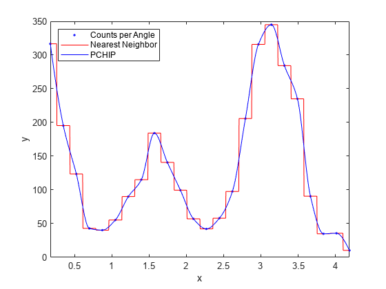
For example, the following plot shows a nearest neighbor interpolant fit and a
shape-preserving (PCHIP) interpolant fit for the nuclear reaction data from the
carbon12alpha.mat sample data set. The nearest neighbor
interpolant is not as smooth as the shape-preserving interpolant.
Note
Goodness-of-fit statistics, prediction bounds, and weights are not defined for interpolants. Additionally, the fit residuals are always 0 (within computer precision) because interpolants pass through the data points.
Biharmonic interpolant fits consist of radial basis function interpolants. All other interpolants supported by Curve Fitting Toolbox are piecewise polynomials and consist of multiple polynomials defined between data points. For cubic spline and PCHIP interpolation, four coefficients describe each piece. Curve Fitting Toolbox uses a cubic (third-degree) polynomial to calculate the four coefficients. Refer to the following for more information:
splinefor cubic spline interpolationpchipfor shape-preserving (PCHIP) interpolation, and for a comparison of PCHIP and cubic spline interpolationscatteredInterpolant,griddata, andtpapsfor surface interpolationIt is possible to fit a single polynomial interpolant to data, with a degree one less than the number of data points. However, the behavior of such fits is unpredictable between data points. Piecewise polynomials with lower-order segments do not diverge significantly from the fitting data domain, so they are useful for analyzing a wider range of data sets.
Selecting an Interpolant Fit
Select Interpolant Fit Interactively
Open the Curve Fitter app by entering curveFitter at the
MATLAB command line. Alternatively, on the Apps tab, in the Math, Statistics and
Optimization group, click Curve Fitter.
On the Curve Fitter tab, in the Fit Type section, select an Interpolant fit. The app fits an interpolating curve or surface that passes through every data point.
In the Fit Options pane, you can specify the Interpolation method value.
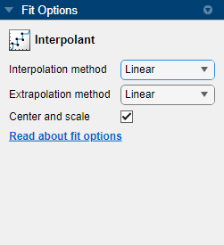
For curve data, you can set Interpolation method to
Linear, Nearest neighbor,
Cubic spline, or Shape-preserving
(PCHIP). For surface data, you can set Interpolation
method to Linear, Nearest
neighbor, Natural neighbor, Cubic
spline, Biharmonic (v4), or Thin-plate
spline.
For surfaces, the Interpolant fit uses the scatteredInterpolant function for
the Linear, Nearest neighbor, and
Natural neighbor methods, the griddata function for the
Cubic Spline and Biharmonic (v4)
methods, and the tpaps function for the
Thin-plate spline method. Try the Thin-plate
spline method when you require both smooth surface interpolation
and good extrapolation properties.
Tip
If your data variables have very different scales, clear the
Center and scale check box to see the
difference in the fit. Normalizing the inputs might influence the
results of the piecewise Linear and Cubic
Spline interpolation methods, and the Nearest
neighbor and Natural neighbor surface
interpolation methods.
Fit Linear Interpolant Model Using the fit Function
Load the census sample data set.
load censusThe variables pop and cdate contain data for the population size and the year the census was taken, respectively.
You can use the fit function to fit any of the interpolant models described in Interpolant Model Names. In this case, fit a linear interpolant model using the 'linearinterp' option, and then plot the result.
f = fit(cdate,pop,'linearinterp');
plot(f,cdate,pop);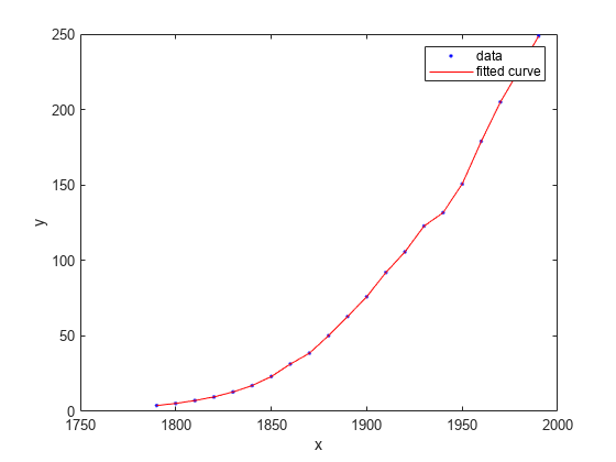
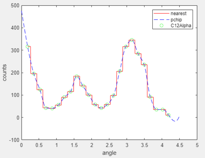
Compare Linear Interpolant Models
Load the carbon12alpha sample data set. Create both nearest neighbor and PCHIP interpolant fits using the 'nearestinterp' and 'pchip' options.
load carbon12alpha
f1 = fit(angle,counts,'nearestinterp');
f2 = fit(angle,counts,'pchip');
Compare the fitted curves f1 and f2 by plotting them in the same figure.
p1 = plot(f1,angle,counts);
xlim([min(angle),max(angle)])
hold on

p2 = plot(f2,'b');
hold off
legend([p1;p2],'Counts per Angle','Nearest Neighbor','PCHIP',...
    'Location','northwest')