Feedback Amplifier Design

Op Amp Description

The standard building block of electrical feedback circuits is the operational amplifier (op amp), a differential voltage amplifier designed to have extremely high dc gain, often in the range of 1e5 to 1e7.

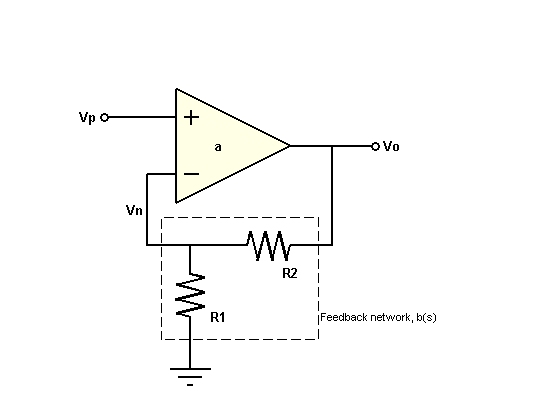
The electrical symbol for the op amp is shown below.

This example assumes the use of an uncompensated op amp with two poles (at frequencies w1,w2) and high dc gain (a0). Assuming this op amp is operated in its linear mode (not saturated), then its open-loop transfer function can be represented as a linear time-invariant (LTI) system, as shown above.

Though higher-order poles exist for a physical op amp, this example assumes that these poles lie in a frequency range where the magnitude is well below unity.

The open-loop transfer functions for this op amp is as follows.

For this example, assume the following transfer function parameters.

a0 = 1e5;
w1 = 1e4;
w2 = 1e6;

Create a transfer function model of this system using a Control System Toolbox LTI model.

First, define the Laplace variable s using the tf command. Then use s to construct the open-loop transfer function a.

s = tf('s');          
a = a0/(1+s/w1)/(1+s/w2)

a =
 
           1e15
  ----------------------
  s^2 + 1.01e06 s + 1e10
 
Continuous-time transfer function.

View the frequency response of this system.

bp = bodeplot(a,'r');
bp.FrequencyUnit = 'rad/s';
bp.MagnitudeUnit = 'dB';
bp.PhaseUnit = 'deg';
bp.YLimits = {[0,110];[-180,0]}

bp = 
  BodePlot with properties:

                 Responses: [1x1 controllib.chart.response.BodeResponse]
           Characteristics: [1x1 controllib.chart.options.CharacteristicsManager]

             FrequencyUnit: "rad/s"
            FrequencyScale: "log"
             MagnitudeUnit: "dB"
            MagnitudeScale: "linear"
                 PhaseUnit: "deg"
          MagnitudeVisible: on
              PhaseVisible: on
      PhaseWrappingEnabled: off
       PhaseWrappingBranch: -180
      PhaseMatchingEnabled: off
    PhaseMatchingFrequency: 0
        PhaseMatchingValue: 0
        MinimumGainEnabled: off
          MinimumGainValue: 0

                   Visible: on
                IOGrouping: "none"
              InputVisible: on
             OutputVisible: on

  Use GET to show all properties

View the normalized step response of a using the stepplot and dcgain commands.

a_norm = a / dcgain(a);
stepplot(a_norm,'r')

title('Normalized Open-Loop Step Response')
ylabel('Normalized Amplitude')

Right-click on the plot and select "Characteristics -> Settling Time" to display the settling time. Hold the mouse over the settling time marker to reveal the exact value of the settling time.

Feedback Amplifier

Now add a resistive feedback network and wire the system as a noninverting amplifier.

This feedback network, b, is simply a voltage divider with input Vo and output Vn. Solving for the ratio Vn/Vo yields the transfer function for b.

     b  =  Vn / Vo  =  R1 / (R1 + R2) 

The block diagram representation of the system is shown below.

Solving for the ratio Vo/Vp yields the closed-loop gain, A.

     A  =  Vo / Vp  =  a / (1 + ab)

If the product of a and b is sufficiently large (>>1), then A can be approximated as:

     A  =  1 / b

Assume that you need to design an amplifier of dc gain (Vo/Vp) 10 and that R1 is fixed at 10 kOhm. Solve for R2.

A0 = 10;
b = 1 / A0;    % approximation for ab>>1
R1 = 10000;
R2 = R1 * (1/b - 1)

R2 = 
90000

Construct the closed-loop system using the feedback command:

A = feedback(a,b);

Plot the frequency responses of a and A together using the bodemag command:

bodemag(a,'r',A,'b');


ylim([0,110]);

% Annotations
opampdemo_annotate(1)
legend('Open-Loop Gain (a)','Closed-Loop Gain (A)','','','','');

The use of negative feedback to reduce the low-frequency (LF) gain has led to a corresponding increase in the system bandwidth (defined as the frequency where the gain drops 3 dB below its maximum value).

This gain versus bandwidth trade off is a powerful tool in the design of feedback amplifier circuits.

Since the gain is now dominated by the feedback network, a useful relationship to consider is the sensitivity of this gain to variation in the op amp's natural (open-loop) gain.

Before deriving the system sensitivity, however, it is useful to define the loop gain, L, which is the total gain a signal experiences traveling around the loop:

L = a * b;

You will use this quantity to evaluate the system sensitivity and stability margins.

The system sensitivity, S, represents the sensitivity of A to variation in a.

The inverse relationship between S and L reveals another benefit of negative feedback, gain desensitivity.

S = 1 / (1 + L);

S has the same form as the feedback equation and, therefore, can be constructed using the more-robust feedback command:

S = feedback(1,L);

The magnitudes of S and A may be plotted together using the bodemag command:

bodemag(A,'b',S,'g')
legend('Closed-Loop Gain(A)','System Sensitivity(S)', ...
    'Location','SouthEast');

The very small low-frequency sensitivity (about -80 dB) indicates a design whose closed-loop gain suffers minimally from open-loop gain variation. Such variation in a is common due to manufacturing variability, temperature change, and so on.

You can check the step response of A using the stepplot command:

stepplot(A)

% Annotation
opampdemo_annotate(2)

The use of feedback has greatly reduced the settling time (by about 98%). However, the step response now displays a large amount of ringing, indicating poor stability margin.

You can analyze the stability margin by plotting the loop gain, L, with the margin command:

margin(L)

The resulting plot indicates a phase margin of less than 6 degrees. You will need to compensate this amplifier in order to raise the phase margin to an acceptable level (generally 45 deg or more), thus reducing excessive overshoot and ringing.

Feedback Lead Compensation

A commonly used method of compensation in this type of circuit is "feedback lead compensation". This technique modifies b(s) by adding a capacitor, C, in parallel with the feedback resistor, R2.

The capacitor value is chosen so as to introduce a phase lead to b near the crossover frequency, thus increasing the amplifier phase margin.

The new feedback transfer function is shown below.

You can approximate a value for C by placing the zero of b at the 0 dB crossover frequency of L:

[Gm,Pm,Wcg,Wcp] = margin(L);
C = 1/(R2*Wcp)

C = 
1.1139e-12

To study the effect of C on the amplifier response, create an LTI model array of b for several values of C around your initial guess:

K = R1/(R1+R2);
C = [1:.2:3]*1e-12;
for n = 1:length(C)
    b_array(:,:,n) = tf([K*R2*C(n) K],[K*R2*C(n) 1]);
end

You can create LTI arrays for A and L.

A_array = feedback(a,b_array);
L_array = a*b_array;

You can plot the step response of all models in the LTI array, A_array, together with A using the stepplot command.

stepplot(A,'b:',A_array,'b',[0:.005:1]*1.5e-6)
title('Closed-Loop Step Response (Compensated)')
        
% Plot Annotations
opampdemo_annotate(3)

The phase margins for our loop gain array, L_array, are found using the margin command.

[Gm,Pm,Wcg,Wcp] = margin(L_array);

The phase margins may now be plotted as a function of C.

plot(C*1e12,Pm,'g')
ax = gca;
xlim([0.8 3.6])
ylim([45 60])
ax.Box = 'on';
xlabel('Compensation Capacitor, C (pF)')
ylabel('Phase Margin (deg)')

% Plot Annotations
opampdemo_annotate(4)

A maximum phase margin of 58 deg is obtained when C = 2 pF (2e-12).

The model corresponding to C = 2 pF is the sixth model in the LTI array, b_array. You can plot the step response of the closed-loop system for this model by selecting index 6 of the LTI array A_array.

A_comp = A_array(:,:,6);
stepplot(A,'b:',A_comp,'b')
legend('Uncompensated (0 pF)','Compensated (2 pF)');

The settling time has been further reduced (by an additional 85%).

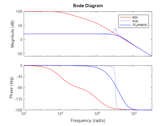
You can overlay the frequency-response of all three models (open-loop, closed-loop, compensated closed-loop) using the bode command:

bodeplot(a,'r',A,'b:',A_comp,'b')
legend('a(s)','A(s)','A\_comp(s)');

The addition of the compensation capacitor eliminates peaking in the closed-loop gain and also greatly extended the phase margin.

Summary

A brief summary of the choice of component values in the design of this non-inverting feedback amplifier circuit: