Discretizing and Resampling Models

Open Script

This example shows how to use the commands for continuous/discrete, discrete/continuous, and discrete/discrete conversions.

Related Commands

Control System Toolbox™ offers extensive support for discretization and resampling of linear systems including:

c2d discretizes continuous-time models
d2c compute continuous-time extensions of discrete-time models
d2d resamples discrete-time models.

Several algorithms are available to perform these operations, including:

Zero-order hold
First-order hold
Impulse invariant
Tustin
Matched poles/zeros.

Continuous/Discrete Conversion

For example, consider the second-order system with delay:

$G(s) = e^{-s} {s - 2 \over s^2 + 3 s + 20}$

To compute its zero-order hold (ZOH) discretization with sampling rate of 10 Hz, type

G = tf([1 -2],[1 3 20],'inputdelay',1);
Ts = 0.1;   % sampling interval
Gd = c2d(G,Ts)

Gd =
 
             0.07462 z - 0.09162
  z^(-10) * ----------------------
            z^2 - 1.571 z + 0.7408
 
Sample time: 0.1 seconds
Discrete-time transfer function.

Compare the continuous and discrete step responses:

step(G,'b',Gd,'r')
legend('Continuous','Discretized')

Discrete/Continuous Conversion

Conversely, you can use d2c to compute a continuous-time "interpolant" for a given discrete-time system. Starting with the discretization Gd computed above, convert it back to continuous and compare with the original model G:

Gc = d2c(Gd);
step(G,'b',Gd,'r',Gc,'g--')
legend('Original','Discretized','D2C Interpolant')

The two continuous-time responses match perfectly. You may not always obtain a perfect match especially when your sampling interval Ts is too large and aliasing occurs during discretization:

Ts = 1;  % 10 times larger than previously
Hd = c2d(G,Ts);
Hc = d2c(Hd);
step(G,'b',Hd,'r',Hc,'g--',10)
legend('Original','Discretized','D2C Interpolant')

Resampling of Discrete-Time Systems

Resampling consists of changing the sampling interval of a discrete-time system. This operation is performed with d2d. For example, consider the 10 Hz discretization Gd of our original continuous-time model G. You can resample it at 40 Hz using:

Gr = d2d(Gd,0.025)

Gr =
 
             0.02343 z - 0.02463
  z^(-40) * ----------------------
            z^2 - 1.916 z + 0.9277
 
Sample time: 0.025 seconds
Discrete-time transfer function.

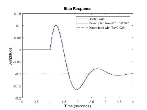
Compare this with a direct discretization at 40 Hz:

step(G,'b',Gr,'r',c2d(G,0.025),'g--',4)
legend('Continuous','Resampled from 0.1 to 0.025','Discretized with Ts=0.025')

Notice that both approaches lead to the same answer.

Which Algorithm and Sampling Rate to Choose?

See the example entitled Discretizing a Notch Filter for more details on how the choice of algorithm and sampling rate affect the discretization accuracy.