Connecting Models

Overview

Control System Toolbox™ provides a number of functions to help you build networks of LTI models. These include functions to perform

These functions can handle any combination of model representations. For illustration purposes, create the following two SISO transfer function models:

H1 = tf(2,[1 3 0])

H1 =
 
      2
  ---------
  s^2 + 3 s
 
Continuous-time transfer function.

H2 = zpk([],-5,5)

H2 =
 
    5
  -----
  (s+5)
 
Continuous-time zero/pole/gain model.

Series Connection

Use the * operator or the series function to connect LTI models in series, for example:

H = H2 * H1

H =
 
       10
  -------------
  s (s+5) (s+3)
 
Continuous-time zero/pole/gain model.

or equivalently

H = series(H1,H2);

Parallel Connection

Use the + operator or the parallel function to connect LTI models in parallel, for example:

H = H1 + H2

H =
 
  5 (s+2.643) (s+0.7566)
  ----------------------
      s (s+3) (s+5)
 
Continuous-time zero/pole/gain model.

or equivalently

H = parallel(H1,H2);

Feedback Connections

The standard feedback configuration is shown below:

To build a model of the closed-loop transfer from u to y, type

H = feedback(H1,H2)

H =
 
              2 (s+5)
  --------------------------------
  (s+5.663) (s^2 + 2.337s + 1.766)
 
Continuous-time zero/pole/gain model.

Note that feedback assumes negative feedback by default. To apply positive feedback, use the following syntax:

H = feedback(H1,H2,+1);

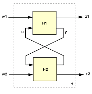
You can also use the lft function to build the more general feedback interconnection sketched below.

Concatenating Inputs and Outputs

You can concatenate the inputs of the two models H1 and H2 by typing

H = [ H1 , H2 ]

H =
 
  From input 1 to output:
     2
  -------
  s (s+3)
 
  From input 2 to output:
    5
  -----
  (s+5)
 
Continuous-time zero/pole/gain model.

The resulting model has two inputs and corresponds to the interconnection:

Similarly, you can concatenate the outputs of H1 and H2 by typing

H = [ H1 ; H2 ]

H =
 
  From input to output...
          2
   1:  -------
       s (s+3)
 
         5
   2:  -----
       (s+5)
 
Continuous-time zero/pole/gain model.

The resulting model H has two outputs and one input and corresponds to the following block diagram:

Finally, you can append the inputs and outputs of two models using:

H = append(H1,H2)

H =
 
  From input 1 to output...
          2
   1:  -------
       s (s+3)
 
   2:  0
 
  From input 2 to output...
   1:  0
 
         5
   2:  -----
       (s+5)
 
Continuous-time zero/pole/gain model.

The resulting model H has two inputs and two outputs and corresponds to the block diagram:

You can use concatenation to build MIMO models from elementary SISO models, for example:

H = [H1 , -tf(10,[1 10]) ; 0 , H2 ]

H =
 
  From input 1 to output...
          2
   1:  -------
       s (s+3)
 
   2:  0
 
  From input 2 to output...
        -10
   1:  ------
       (s+10)
 
         5
   2:  -----
       (s+5)
 
Continuous-time zero/pole/gain model.

sigma(H), grid

Building Models from Block Diagrams

You can use combinations of the functions and operations introduced so far to construct models of simple block diagrams. For example, consider the following block diagram:

with the following data for the blocks F, C, G, S:

s = tf('s');
F = 1/(s+1);
G = 100/(s^2+5*s+100);
C = 20*(s^2+s+60)/s/(s^2+40*s+400);
S = 10/(s+10);

You can compute the closed-loop transfer T from r to y as

T = F * feedback(G*C,S);
step(T), grid

For more complicated block diagrams, the connect function provides a systematic and simple way to wire blocks together. To use connect, follow these steps:

For the block diagram above, these steps amount to:

Sum1 = sumblk('e = r - y');
Sum2 = sumblk('u = uC + uF');

% Define block I/Os ("u" and "y" are shorthand for "InputName" and "OutputName")
F.u = 'r';   F.y = 'uF';
C.u = 'e';   C.y = 'uC';
G.u = 'u';   G.y = 'ym';
S.u = 'ym';  S.y = 'y';

% Compute transfer r -> ym
T = connect(F,C,G,S,Sum1,Sum2,'r','ym');
step(T), grid

Precedence Rules

When connecting models of different types, the resulting model type is determined by the precedence rule

  FRD > SS > ZPK > TF > PID

This rule states that FRD has highest precedence, followed by SS, ZPK, TF, and PID has the lowest precedence. For example, in the series connection:

H1 = ss(-1,2,3,0);
H2 = tf(1,[1 0]);
H = H2 * H1;

H2 is automatically converted to the state-space representation and the result H is a state-space model:

class(H)

ans = 
'ss'

Because the SS and FRD representations are best suited for system interconnections, it is recommended that you convert at least one of the models to SS or FRD to ensure that all computations are performed using one of these two representations. One exception is when using connect which automatically performs such conversion and always returns a state-space or FRD model of the block diagram.