Compute Acoustic Room Transfer Function with Finite Element Analysis

Since R2026a

Sound fields within small rooms and enclosures are dominated by standing waves and modal behavior, particularly at low frequencies. In this scenario, geometric simulation methods, such as ray tracing, are unreliable. The recommended approach is to use a wave-based solver, such as the finite element method (FEM).

This example computes the room transfer function between a source and a receiver using FEM provided by Partial Differential Equation Toolbox™. The example follows these steps:

1. Determine the room response at a target frequency assuming a point-source location.

2. Evaluate the source-to-receiver transfer function over a frequency range for a specified receiver location.

3. Compare the simulated transfer function to a theoretical reference based on the Green function for a rectangular room.

4. Simulate the frequency transfer function for a nonrectangular room.

Determine Rectangular Room Response at Target Frequency

Specify Target Frequency

Specify the speed of sound.

c0 = 343;

Specify the frequency at which you want to run the analysis, in hertz.

targetFrequency = 114;

Specify the wave number corresponding to the selected frequency.

k = 2*pi*targetFrequency/c0;

Model Rectangular Room

Create and visualize a shoe-box room with desired width (W), depth (D), and height (H) in meters.

W = 1.9;
D = 1.7;
H = 1.5;
room = multicuboid(W,D,H);

Move the corner of the room geometry to (0,0,0).

room = translate(room,[W/2 D/2 0]);
figure
pdegplot(room,CellLabels="on",FaceAlpha=0.5)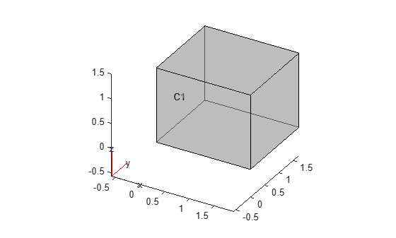

Assign surface absorption coefficients to each room wall. These coefficients represent the fraction of acoustic energy absorbed by each surface (values between 0 and 1). Assume that the walls are highly reflecting.

To simplify the example, assume all surfaces have the same absorption coefficient.

alpha = .1;

Compute the equivalent normalized specific wall admittance.

beta = (1-sqrt(1-alpha))/(1+sqrt(1-alpha));

Create the PDE model and set its geometry to the empty room.

model = createpde;
model.Geometry = room;

The boundary conditions for nonrigid walls in a rectangular room are defined in [1]:

• $\frac{dp}{dx}-1jk\frac{p}{\zeta }=0$ for the wall defined by x=0.

• $\frac{dp}{dx}+1jk\frac{p}{\zeta }=0$ for the wall defined by x=W.

p is the acoustic pressure, and $\zeta$ is the specific wall impedance (the reciprocal of the admittance). The boundary conditions of the other walls are derived in a similar fashion.

The model defines generalized Neumann conditions of the form: $n\cdot \left(c\times \nabla p\right)+qp=g$. Apply the boundary condition by matching q and g to the desired values. Note that you drop the -1 factors that appear for certain walls in the equations because Partial Differential Equation Toolbox uses the outward normal derivative in the boundary conditions.

for faceID =1:model.Geometry.NumFaces
    h_i = 1i*k*beta;
    applyBoundaryCondition(model,"neumann",Face=1:room.NumFaces,q=h_i,g=0);
end

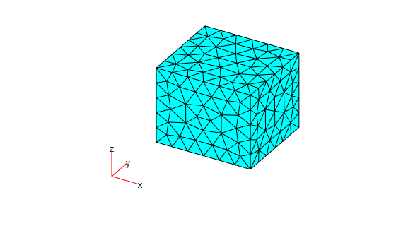
FEM is based on meshing, which divides a complex geometry into smaller, simpler elements. Typically, the element size must be 1/10th of the wavelength of the highest frequency of interest. The wavelength is given by $\lambda =\frac{c_0}{f},$where f is the frequency, in hertz. Define the mesh size.

meshSize = (c0/targetFrequency)/10;

Create and plot a mesh for the room geometry.

msh = generateMesh(model,Hmax=meshSize);
pdemesh(msh)

Define Point Source and PDE Coefficients

Start by analyzing the received pressure in different points in the room. In acoustics, a true point source is represented mathematically by a Dirac delta function, which is an idealized impulse concentrated at a single point. However, the delta function is not suitable for a numerical simulation due to its infinite amplitude and zero width. Instead, approximate a point source with a narrow 3-D Gaussian function centered at the specified source location. The Gaussian is spatially localized and smoothly decays away from the source point. Its width is controlled by the standard deviation sigma (in meters).

Choose sigma small enough compared to the acoustic wavelength (so the source behaves like a point), but not so small that it falls below the mesh resolution. This expression ensures the Gaussian is narrow (about 1/30 of a wavelength), but still resolvable by the mesh.

sigma = max(meshSize,(c0/targetFrequency)/30)/2;

Specify the coordinates of the point source in the room.

src = [0.31*W 0.47*D 0.63*H];

Specify the source strength function using a normalized Gaussian profile centered at src, with normalization chosen so that its total integral equals 1. This function returns the spatial source amplitude at any point in the mesh.

normC = 1/((2*pi)^(3/2)*sigma^3); % normalizing factor
Q_fun = @(loc,~) reshape(normC*exp(-((loc.x-src(1)).^2+ ...
                                     (loc.y-src(2)).^2+ ...
                                     (loc.z-src(3)).^2)/(2*sigma^2)),1,[]);

To specify the PDE coefficients, compare the inhomogeneous Helmholtz equation defined in [2]:

$${\nabla }^{2}p\left(r,r_0\right)+k^{2}p\left(r,r_0\right)=-\delta \left(r-r_0\right)$$

with the equation form expected by the PDE model:

$$m\frac{{\delta }^{2}u}{\delta t^2}+d\frac{\delta u}{\delta t}-\nabla .\left(c\nabla u\right)+au=f.$$

Here, $r_0$ represents the source location. Use specifyCoefficients to specify the coefficients accordingly.

specifyCoefficients(model,m=0,d=0,c=1,a=-k^2,f=Q_fun);

Simulate and Visualize Room Pressure

Solve the Helmholtz equation.

result = solvepde(model);

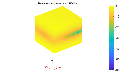
Visualize the pressure level on the room surfaces.

U = result.NodalSolution;                 % complex pressure at mesh nodes
PLdB = mag2db(abs(U)/max(abs(U)));        % relative level in dB (re max)

figure
pdeplot3D(model, ColorMapData=PLdB)
colorbar
clim([-60 0])
title("Pressure Level on Walls")
view(3)
axis equal tight
colormap parula

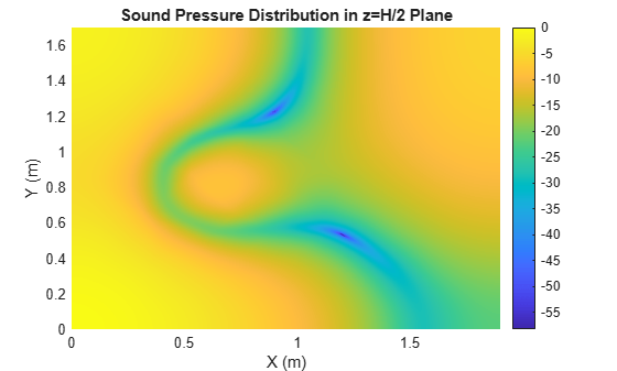
Visualize the pressure on the horizontal plane, z = H/2, by interpolating the results for this plane.

xx = 0:W/200:W;
yy = 0:D/200:D;
[XX,YY] = meshgrid(xx,yy);
ZZ = (H/2)*ones(size(XX));

Vq = interpolateSolution(result,XX,YY,ZZ);
Vq = reshape(Vq,size(XX));
Vq = abs(Vq);
Vq = Vq./max(Vq(:));

figure
surface(xx,yy,20*log10(Vq))
colorbar
shading interp
xlabel("X (m)")
ylabel("Y (m)")
axis tight
title("Sound Pressure Distribution in z=H/2 Plane")

View the plane pressure distribution in 3-D.

figure
visualizePressureInPlane3D(W,D,H,XX,YY,ZZ,mag2db(Vq))
title("Sound Pressure Distribution in z=H/2 Plane")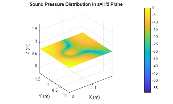

Generate Frequency-Domain Transfer Function

Compute the room transfer function over a frequency range assuming a specific receiver location.

Specify the receiver location.

rx = [0.73*W 0.61*D 0.41*H];

Specify the frequency range.

FVect = linspace(20,200,20);

Preallocate the pressure response vector.

G_sim = zeros(1,numel(FVect));

Specify the mesh size based on the largest desired frequency.

meshSize = (c0/FVect(end))/10;

Specify the source based on the largest desired frequency.

sigma = max(meshSize,(c0/FVect(end))/30)/2;
normC = 1/((2*pi)^(3/2)*sigma^3);
Q_fun = @(loc,~) reshape(normC*exp(-((loc.x-src(1)).^2+ ...
                                     (loc.y-src(2)).^2+ ...
                                     (loc.z-src(3)).^2)/(2*sigma^2)),1,[]);

Compute the received pressure for each frequency point. The iteration steps are similar to the workflow of the previous section:

1. Select the frequency point.

2. Derive the equivalent wave number.

3. Apply the surface boundary conditions.

4. Specify the coefficients.

5. Solve the Helmholtz equation.

6. Interpolate the results to the receiver position.

for index = 1:numel(FVect)
    f = FVect(index);
    k = 2*pi*f/c0; % wave number
    applyBoundaryCondition(model,"neumann", ...
        Face=1:model.Geometry.NumFaces,q=1i*k*beta,g=0);
    specifyCoefficients(model,m=0,d=0,c=1,a=-k^2,f=Q_fun);
    result = solvepde(model);
    G_sim(index) = interpolateSolution(result,rx(1),rx(2),rx(3));
end

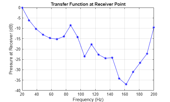
Normalize and plot the received pressure.

G_sim = abs(G_sim);
G_sim = G_sim/max(G_sim(:));

figure
plot(FVect,mag2db(abs(G_sim+realmin)),"b*-")
title("Transfer Function at Receiver Point")
xlabel("Frequency (Hz)")
ylabel("Pressure at Receiver (dB)")
hold on
grid on

Compare Simulation to Theoretical Green's Function

View Transfer Function Over Simulation Frequency Range

Compare the simulation results to the theoretical response for a rectangular room given by the Green's function. Green's function for a shoe-box room is defined in [2] as follows:

$p\left(r,r_0\right)=-\frac{c_0^2}{V{\left(2\pi \right)}^2}\sum _m\frac{{\psi }_m\left(r\right){\psi }_m\left(r_0\right)}{f^2-f_m^2-1j\frac{f}{2\pi {\tau }_m}}$.

• $p\left(r,r_0\right)$is the acoustic pressure at point r due to the source at $r_0.$

• $c_0$is the speed of sound (in meters per second).

• V is the room volume (in cubic meters).

• f is the target frequency (in hertz).

• $f_m$is the m-th modal frequency.

• ${\psi }_m\left(r\right)$is the normalized mode shape function at r.

• ${\tau }_m$is the modal decay time constant.

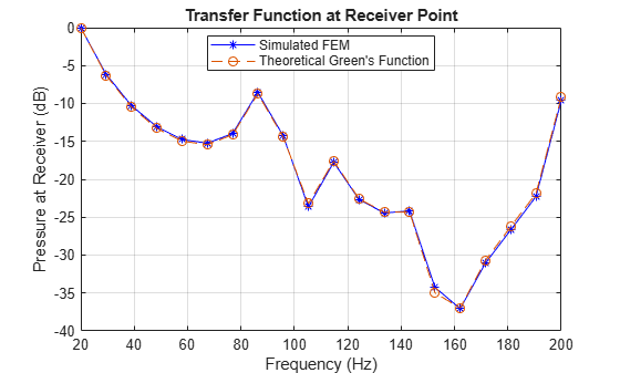
Generate the theoretical response and compare it to the simulated results. The helper function greenFunction computes the theoretical received pressure by including the contributions of the axial, tangential and oblique modes.

G = greenFunction([W D H],src,rx,FVect,c0,alpha);
G = abs(G);
G = G/max(G(:));

plot(FVect,mag2db(abs(G+realmin)),"--o")
legend({"Simulated FEM","Theoretical Green's Function"},Location="best")

View Transfer Function Up To Schroeder Frequency

Depending on the enclosure characteristics, modal behavior can dominate, and therefore, FEM simulation is required over a wider frequency range. The Schroeder frequency, also known as the transition frequency, is a point in the audio spectrum where sound wave behavior shifts from being dominated by room resonances (or modal behavior) to being more diffuse (or reverberant). You restrict finite-element analysis to frequencies below the Schroeder frequency. For frequencies above the Schroeder frequency, you can use faster geometric simulation techniques, such as ray tracing.

The Schroeder frequency (in hertz) is

$F_T=\frac{2000\sqrt{{\text{RT}}_{60}}}{V}$,

where RT is the room reverberation time (in seconds), and V is the room volume. Compute RT using Sabine's formula:

${RT}_{60}=0.161\frac{V}{A}$,

where A is the is the total absorption in the room in square meters of sabins:

$A=\sum \left({\alpha }_i.S_i\right)$.

Here, ${\alpha }_i$ is the absorption coefficient of the i-th surface, and$S_i$ is the area of the i-th surface.

Compute the room volume.

V = W*D*H;

Compute the total absorption in the room.

A = alpha*(2*W*D + 2*W*H + 2*D*H);

Compute the reverberation time.

RT60 = 0.161*V/A

RT60 = 
0.4519

Compute the Schroeder frequency of the room.

schroederFrequency = 2000*sqrt(RT60/V)

schroederFrequency = 
610.8331

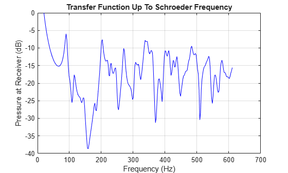
Load the simulation results for a frequency range extending up schroederFrequency. These results were computed with a mesh size of 0.1.

load("FEMFreqRes.mat","FVect","G_sim")

G_sim = abs(G_sim);
G_sim = G_sim/max(G_sim(:));

Plot the simulated frequency response.

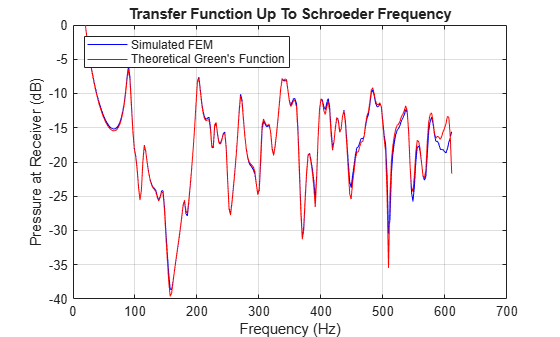
figure
plot(FVect,mag2db(abs(G_sim+realmin)),"b-")
title("Transfer Function Up To Schroeder Frequency")
xlabel("Frequency (Hz)")
ylabel("Pressure at Receiver (dB)")
hold on
grid on

Compare the simulated results to the theoretical Green's function over the same frequency range.

G_green = greenFunction([W D H],src,rx,FVect,c0,alpha);
G_green = abs(G_green);
G_green = G_green/max(G_green(:));

plot(FVect,mag2db(abs(G_green+realmin)),"r-")
legend({"Simulated FEM","Theoretical Green's Function"},Location="northwest")

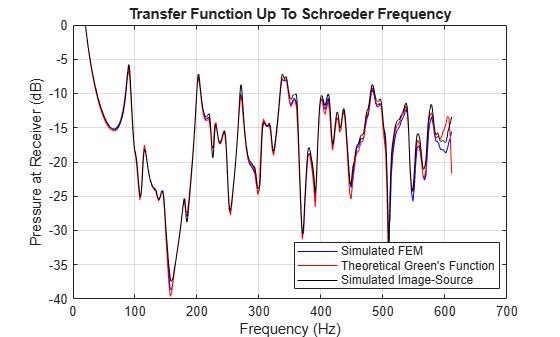
Typically, geometric simulation methods are not suitable for low frequencies. However, for the special case of a rectangular room, the image-source method approaches theoretical results for high orders. The acousticRoomResponse function implements the image-source method.

The function uses the angle-averaged (random incidence) absorption coefficient. Equation (2.42) in [1] expresses the random-incidence coefficient as:

$${\alpha }_{uni}=\frac{8}{{\left|\xi \right|}^2}\cos \mu \left[\left|\xi \right|+\frac{cos2\mu }{\sin \mu }\arctan \left(\frac{\left|\xi \right|\sin \mu }{1+\left|\xi \right|\cos \mu }\right)-\cos \mu \ln \left(1+2\left|\xi \right|\cos \mu +{\left|\xi \right|}^2\right)\right]$$

• $\xi$is the complex surface impedance (the reciprocal of beta).

• $\mu$ is the impedance phase angle.

In this example, the wall is purely resistive, which means that the impedance is real-valued, and $\mu$ approaches zero. As $\mu$$\to$1, the equation becomes:

${\alpha }_{uni}\to \frac{8}{{\left|\xi \right|}^2}\left[\left|\xi \right|+\frac{1}{\mu }\frac{\left|\xi \right|\mu }{1+\left|\xi \right|}-\ln \left({\left(1+\left|\xi \right|\right)}^2\right)\right]$,

${\alpha }_{uni}\to \frac{8}{{\left|\xi \right|}^2}\left[\left|\xi \right|+\frac{\left|\xi \right|}{1+\left|\xi \right|}-2\ln \left(1+\left|\xi \right|\right)\right]$,

${\alpha }_{uni}\to \frac{8}{{\left|\xi \right|}^2}\left[\frac{\left|\xi \right|\left(2+\left|\xi \right|\right)}{1+\left|\xi \right|}-2\ln \left(1+\left|\xi \right|\right)\right]$.

${\alpha }_{uni}$ can be then expressed in terms of the admittance as:

${\alpha }_{uni}=8\beta \left[\frac{1+2\beta }{1+\beta }+2\beta \ln \left(\frac{\beta }{1+\beta }\right)\right]$.

Compute the random-incidence absorption based on this equation:

alpha_diff = 8*beta*((1 + 2*beta)/(1 + beta) + ...
             2*beta*log(beta/(1+beta)));

Compute the room impulse response using acousticRoomResponse. Specify an image-source order of 70. Use the value of alpha_diff to specify surface absorption.

fs = 16e3; % Sample rate
ir = acousticRoomResponse([W D H],src,rx,...
                          MaterialAbsorption=alpha_diff,...
                          Algorithm="image-source",...
                          ImageSourceOrder=70,...
                          SampleRate=fs);

Compute the frequency response from the impulse response.

[G,F] = freqz(ir,1,2^18,fs);

Select and normalize the part of the response that corresponds to the frequency range over which FEM simulation was executed.

FVect = F(F>=20 & F<=schroederFrequency);
G = abs(G(F>=20 & F<=schroederFrequency));
G = G/max(G);

Overlay the image-source simulation response over the FEM and theoretical responses.

plot(FVect,mag2db(abs(G+realmin)),"k-")
legend({"Simulated FEM", ...
        "Theoretical Green's Function", ...
        "Simulated Image-Source"}, ...
        Location="best")

Simulate Pressure for Nonrectangular Room

Simulate the transfer function of a nonrectangular room by using the same approach that you used for a rectangular room. First, import the geometry of a nonrectangular room.

gm = importGeometry("customRoom.stl");
model.Geometry = gm;

Visualize the room.

figure
pdegplot(model,FaceAlpha=0.2,FaceLabels="on")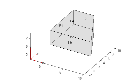

Specify the coordinates of the source, in meters.

src = [2.5,5.1,1.85];

Specify the coordinates of the receiver, in meters.

receiver = [3.75,7.8,2.2];

Specify the absorption coefficient for each surface.

alpha = 1e-3*[1 1.5 2 2.5 1.1 1.7];

Compute the equivalent normalized specific admittance for each surface.

beta = (1-sqrt(1-alpha))./(1+sqrt(1-alpha));

Specify the frequency range.

FVect = linspace(20,100,20);

Specify the mesh size based on the largest desired frequency.

meshSize = (c0/FVect(end))/5;

Generate the mesh.

generateMesh(model,Hmax=meshSize);

Specify the source based on the largest frequency.

sigma = max(meshSize,(c0/FVect(end))/30)/2;
normC = 1/((2*pi)^(3/2)*sigma^3);
Q_fun = @(loc,~) reshape(normC*exp(-((loc.x-src(1)).^2+ ...
                                     (loc.y-src(2)).^2+ ...
                                     (loc.z-src(3)).^2)/(2*sigma^2)),1,[]);

Specify the pressure response vector.

G_sim = zeros(1,numel(FVect));

Compute the received pressure for each frequency point.

for index = 1:numel(FVect)

    f = FVect(index);
    k = 2*pi*f/c0; % wave number

    for faceID = 1:model.Geometry.NumFaces
        h_i = 1i*k*beta(faceID);
        applyBoundaryCondition(model,"neumann",Face=faceID,q=h_i,g=0);
    end
   
    specifyCoefficients(model,m=0,d=0,c=1,a=-k^2,f=Q_fun);
    result = solvepde(model);

    % Interpolate to the receiver point
    G_sim(index) = interpolateSolution(result, rx(1), rx(2), rx(3));
end

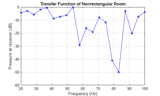
Normalize and plot the received pressure.

G_sim = abs(G_sim);
G_sim = G_sim/max(G_sim(:));

figure
plot(FVect,mag2db(abs(G_sim+realmin)),"b*-")
title("Transfer Function of Nonrectangular Room")
xlabel("Frequency (Hz)")
ylabel("Pressure at receiver (dB)")
hold on
grid on

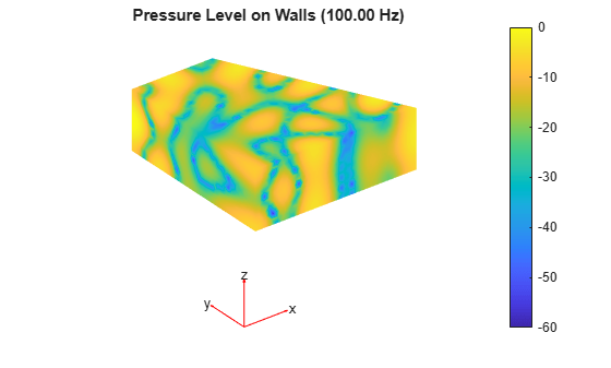
Visualize the pressure level on the room surfaces for the largest simulated frequency.

U = result.NodalSolution;        
PLdB = 20*log10(abs(U)/max(abs(U)));  

figure
pdeplot3D(model,ColorMapData=PLdB)
colorbar
clim([-60 0])
title(sprintf("Pressure Level on Walls (%0.2f Hz)",FVect(end)))
view(3)
axis equal tight
colormap parula

Helper Functions

function visualizePressureInPlane3D(L,W,H,XX,YY,ZZ,Vq)
% Visualize the pressure in a plane in 3-D
% L, W, H: Room dimensions
% Xx, YY, ZZ: mesh grids
% Vq: Output of interpolateSolution

% Outline the 3D room from (0,0,0) to (L,W,H)
V = [0 0 0;
    L 0 0;
    L W 0;
    0 W 0;
    0 0 H;
    L 0 H;
    L W H;
    0 W H];
E = [1 2;2 3;3 4;4 1; 5 6;6 7;7 8;8 5; 1 5;2 6;3 7;4 8];
for e=1:size(E,1)
    plot3(V(E(e,:),1),V(E(e,:),2),V(E(e,:),3),"k-",LineWidth=1);
end

% Surface plot of the slice
surf(XX,YY,ZZ,Vq,EdgeColor="none");
shading interp;
colorbar;
xlabel("X (m)"); ylabel("Y (m)"); zlabel("Z (m)");
axis([0 L 0 W 0 H]); axis equal;
view(3);

end

function G = greenFunction(roomDims,tx,rx,freq,c,A)
% Compute analytical Green's function for a lightly damped rectangular room
%
% roomDims: [W D H]  (meters)
% tx, rx   : [x y z] (meters)
% freq     : vector of frequencies (Hz)
% c        : speed of sound (m/s)
% A        : average surface absorption coefficient

W = roomDims(1);  
D = roomDims(2);  
H = roomDims(3);
V = W*D*H;
S = 2*(W*D + W*H + D*H);

% Compute Schroeder frequency
FShroeder = computeShroederFrequency(roomDims,A);
% Schroeder wave number
kS = 2*pi*FShroeder/c;     

% Cap order for each axis
Nx = max(1,floor(kS*W/pi));
Ny = max(1,floor(kS*D/pi));
Nz = max(1,floor(kS*H/pi));

% Compute normalized wall admittance
beta = (1 - sqrt(1 - A))/(1 + sqrt(1 - A));
betaR = real(beta);

K = 2*pi*freq/c;

G = zeros(1,numel(freq));

% Axial contributions
G = G + greenFunctionAxial(W,c,V,S,betaR,tx(1),rx(1),freq,K,Nx);
G = G + greenFunctionAxial(D,c,V,S,betaR,tx(2),rx(2),freq,K,Ny);
G = G + greenFunctionAxial(H,c,V,S,betaR,tx(3),rx(3),freq,K,Nz);

% Tangential contributions
G = G + greenFunctionTangential(FShroeder,W,D,c,V,S,betaR,tx(1:2),rx(1:2),freq,K,[Nx Ny]);
G = G + greenFunctionTangential(FShroeder,W,H,c,V,S,betaR,tx([1 3]),rx([1 3]),freq,K,[Nx Nz]);
G = G + greenFunctionTangential(FShroeder,D,H,c,V,S,betaR,tx([2 3]),rx([2 3]),freq,K,[Ny Nz]);

% Oblique contributions
G = G + greenFunctionOblique(FShroeder,W,D,H,c,V,S,betaR,tx,rx,freq,K,[Nx Ny Nz]);

% Add zero mode (nx = 0, ny = 0, nz = 0)
% See Example 8.3 in [2]
G = G - 1./(V.*K.^2);
end

function G = greenFunctionAxial(W,c,V,S,beta,tx,rx,freq,K,Nx)
% Axial modes contributions to the Green's function
%
% W: dimensions length (m)
% c: speed of sound (m/s)
% V: Room volume (m3)
% S: total surface area (m2)
% beta: normalized wall admittance
% tx, rx: transmitter and receiver locations
% freq: target frequency (Hz)
% K: Wave number
% Nx: Mode order/index

A   = 2; % (8.11) in [2], only one index is nonzero    
tau = 3*V/(4*c*S*beta); % (8.75) in [2]     

% Compute eigen-function values at receiver and transmitter
n = 1:Nx;
phi_tx = sqrt(A)*cos(n*pi*tx/W);
phi_rx = sqrt(A)*cos(n*pi*rx/W);
Km = pi*(n/W);

% Compute Green's function at each frequency
eta = 1e-4;  % small numerical guard 
G = zeros(1,numel(freq));
for i = 1:numel(freq)
    Ki = K(i);
    % Equation (8.35) in [2]
    denom = (Ki^2 - Km.^2) + 1j*(Ki/(tau*c) + 2*eta*Ki);
    vals = (-1/V)*(phi_tx.*phi_rx)./denom;
    G(i) = sum(vals);
end
end

function G = greenFunctionTangential(Fs,W,D,c,V,S,beta,tx,rx,freq,K,Nxy)
% Tangential modes contributions to the Green's function
%
% Fs: Schroeder frequency
% W, D: dimensions length (m)
% c: speed of sound (m/s)
% V: Room volume (m3)
% S: total surface area (m2)
% beta: normalized wall admittance
% tx, rx: transmitter and receiver locations
% freq: target frequency (Hz)
% K: Wave number
% Nxy: Mode indices

Nx = Nxy(1); 
Ny = Nxy(2);
A = 4;                                     % (8.11) in [2]
tau = 3*V/(5*c*S*real(beta));              % (8.75) in [2]

[nx,ny] = ndgrid(1:Nx,1:Ny);
phi_tx = sqrt(A)*cos(nx*pi*tx(1)/W).*cos(ny*pi*tx(2)/D);
phi_rx = sqrt(A)*cos(nx*pi*rx(1)/W).*cos(ny*pi*rx(2)/D);
Km = pi*sqrt((nx/W).^2 + (ny/D).^2);

kS = 2*pi*Fs/c; % Schroeder k-sphere cutoff
mask = (Km<=kS);

eta = 1e-4;
G = zeros(1,numel(freq));
for i = 1:numel(freq)
    Ki = K(i);
    denom = (Ki^2 - Km.^2) + 1j*(Ki/(tau*c) + 2*eta*Ki);
    vals = (-1/V)*(phi_tx.*phi_rx)./denom;
    vals(~mask) = 0;
    G(i) = sum(vals,"all");
end
end

function G = greenFunctionOblique(Fs,W,D,H,c,V,S,beta,tx,rx,freq,K,Nxyz)
% Oblique modes contributions to the Green function
%
% Fs: Schroeder frequency
% W, D, H: dimensions length (m)
% c: speed of sound (m/s)
% V: Room volume (m3)
% S: total surface area (m2)
% beta: normalized wall admittance
% tx, rx: transmitter and receiver locations
% freq: target frequency (Hz)
% K: Wave number
% Nxy: Mode indices

Nx = Nxyz(1);
Ny = Nxyz(2);
Nz = Nxyz(3);
A = 8; % (8.11) in [2]
tau = V/(2*c*S*real(beta)); % (8.75) in [2]

[nx,ny,nz] = ndgrid(1:Nx,1:Ny,1:Nz);
phi_tx = sqrt(A)*cos(nx*pi*tx(1)/W).*cos(ny*pi*tx(2)/D).*cos(nz*pi*tx(3)/H);
phi_rx = sqrt(A)*cos(nx*pi*rx(1)/W).*cos(ny*pi*rx(2)/D).*cos(nz*pi*rx(3)/H);
Km = pi*sqrt((nx/W).^2 + (ny/D).^2 + (nz/H).^2);

kS = 2*pi*Fs/c;
mask = (Km<=kS);

eta = 1e-4;
G = zeros(1,numel(freq));
for i = 1:numel(freq)
    Ki = K(i);
    denom = (Ki^2 - Km.^2) + 1j*(Ki/(tau*c) + 2*eta*Ki);
    vals = (-1/V)*(phi_tx.*phi_rx)./denom;
    vals(~mask) = 0;
    G(i) = sum(vals,"all");
end
end

function FShroeder = computeShroederFrequency(roomDims,absorb)
% Compute Shroeder frequency (Hz)
V = prod(roomDims);
W = roomDims(1);
D = roomDims(2);
H = roomDims(3);
A = absorb*(2*W*D + 2*W*H + 2*D*H);
RT60 = .161*V/A;

FShroeder = 2000*sqrt(RT60/V);
end

References

[1] Kuttruff, Heinrich. Room Acoustics. Sixth edition, CRC Press, 2016.

[2] Jacobsen, Finn, and Peter Moller Juhl. Fundamentals of General Linear Acoustics. John Wiley & Sons Inc., 2013.