Antenna Modeling and Analysis

R2026b

This example shows how to create, visualize, and analyze the antenna elements in the Antenna Toolbox™.

Define Antenna Element Using Antenna Catalog

Define a helix antenna using the helix antenna element from the antenna catalog.

hx = helix

hx = 
  helix with properties:

               Radius: 0.0220
                Width: 1.0000e-03
                Turns: 3
              Spacing: 0.0350
     WindingDirection: 'CCW'
       FeedStubHeight: 1.0000e-03
    GroundPlaneRadius: 0.0750
            Substrate: [1×1 dielectric]
            Conductor: [1×1 metal]
                 Tilt: 0
             TiltAxis: [1 0 0]
                 Load: [1×1 lumpedElement]

Visualize Antenna Geometry

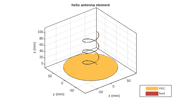
Use the show function to visualize helix antenna geometry. A helix antenna consists of a helical shaped conductor on a ground plane. The ground plane of the antenna is in the xy-plane.

show(hx)

Figure contains an axes object. The axes object with title helix antenna element, xlabel x (mm), ylabel y (mm) contains 4 objects of type patch, surface. These objects represent PEC, feed.

Set Antenna Properties

Set the helix antenna properties as follows:

Radius = 28e-3 m
Width = 1.2e-3 m
Number of Turns = 4

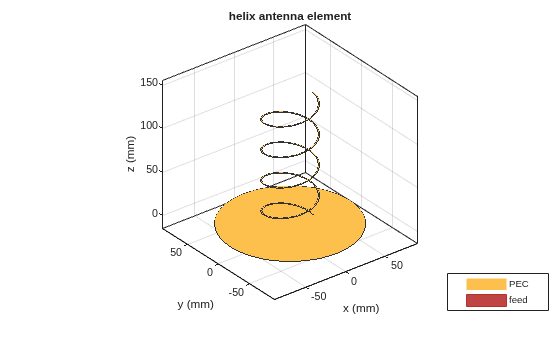
After applying these properties, view the antenna to observe the resulting structural changes.

hx = helix(Radius=28e-3,Width=1.2e-3,Turns=4)

hx = 
  helix with properties:

               Radius: 0.0280
                Width: 0.0012
                Turns: 4
              Spacing: 0.0350
     WindingDirection: 'CCW'
       FeedStubHeight: 1.0000e-03
    GroundPlaneRadius: 0.0750
            Substrate: [1×1 dielectric]
            Conductor: [1×1 metal]
                 Tilt: 0
             TiltAxis: [1 0 0]
                 Load: [1×1 lumpedElement]

show(hx)

Figure contains an axes object. The axes object with title helix antenna element, xlabel x (mm), ylabel y (mm) contains 4 objects of type patch, surface. These objects represent PEC, feed.

Plot 3-D Radiation Pattern

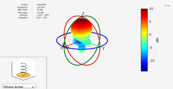
Use the pattern function to plot the radiation pattern for the helix antenna. The radiation pattern of an antenna is its spatial distribution of power. The pattern displays the directivity or gain of the antenna. By default, the pattern function plots the directivity of the antenna.

pattern(hx,1.8e9)

Figure contains 2 axes objects and other objects of type uilabel, uicontrol. Axes object 1 contains 4 objects of type patch, surface. Hidden axes object 2 contains 17 objects of type surface, line, text, patch.

Plot Azimuth and Elevation Pattern

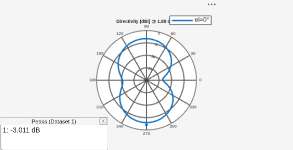
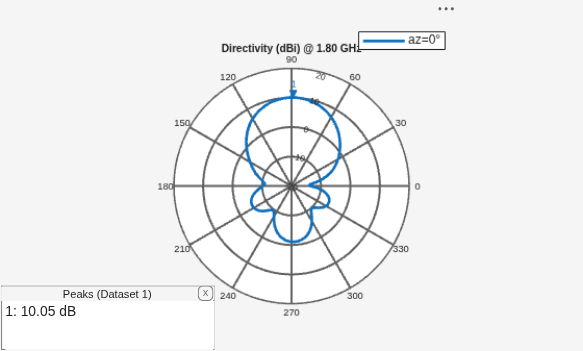
Use patternAzimuth and patternElevation functions to plot the azimuth and elevation pattern of the helix antenna. This is the 2D radiation pattern of the antenna at a specified frequency.

patternAzimuth(hx,1.8e9)

Figure contains an axes object and an object of type uicontainer. The hidden axes object contains 2 objects of type line, text. This object represents el=0° .

figure
patternElevation(hx,1.8e9)

Figure contains an axes object and an object of type uicontainer. The hidden axes object contains 2 objects of type line, text. This object represents az=0° .

Calculate Directivity

Specify an output argument in the pattern function to calculate the directivity of helix antenna. Directivity is the ability of an antenna to radiate power in a particular direction. It can be defined as ratio of maximum radiation intensity in the desired direction to the average radiation intensity in all other directions. The antenna gain and directivity are evaluated in the far-field region. By default, Antenna Toolbox™ uses a radius of 100λ for pattern visualization. However, the far-field condition depends on the antenna size and operating wavelength, and the required distance may vary accordingly.

Directivity = pattern(hx,1.8e9,0,90)

Directivity = 
10.0440

Calculate Electric and Magnetic Fields

Use the EHfields function to calculate the electric and magnetic fields of the helix antenna. The EHfields function outputs the x-, y-, and *z-*components of electric and magnetic fields of an antenna. These components are measured at a specific frequency and at specified points in space.

[E,H] = EHfields(hx,1.8e9,[0;0;1]);

Plot Radiation Pattern for Different Polarization

Use the Polarization name-value argument in the pattern function to plot the radiation pattern of the helix antenna for different polarization. Polarization is the orientation of the electric field, or E-field, of an antenna. Polarization is classified as elliptical, linear, or circular. This example shows the Right-Hand Circularly Polarized (RHCP) radiation pattern of the helix.

pattern(hx,1.8e9, Polarization="RHCP")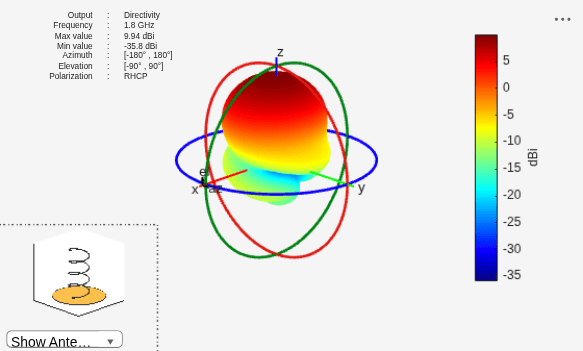

Calculate Axial Ratio

Use the axialRatio function to calculate the axial ratio of the helix antenna. Antenna axial ratio (AR) in a given direction quantifies the ratio of two orthogonal field components radiated in a circularly polarized wave. An axial ratio of infinity, implies a linearly polarized wave. The unit of measure is dB.

ar = axialRatio(hx,1.8e9,20,30)

ar = 
23.8947

Calculate Beamwidth

Use the beamwidth function to calculate the beamwidth of the antenna. Antenna beamwidth is the angular measure of the antenna pattern coverage. Beamwidth angle is measured in plane containing the direction of main lobe of the antenna.

[bw,angles] = beamwidth(hx,1.8e9,0,1:1:360)

bw = 
57.0000

angles = 1×2

    60   117

Calculate Impedance

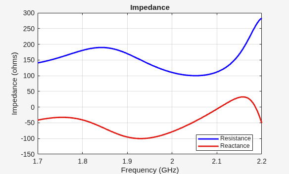
Use the impedance function to calculate and plot the input impedance of helix antenna. Input impedance is a ratio of voltage and current at the port. Antenna impedance is calculated as the ratio of the phasor voltage (which is 1V at a phase angle of 0 deg as mentioned earlier) and the phasor current at the port.

impedance(hx,1.7e9:1e6:2.2e9)

Figure contains an axes object. The axes object with title Impedance, xlabel Frequency (GHz), ylabel Impedance (ohms) contains 2 objects of type line. These objects represent Resistance, Reactance.

Calculate Reflection Coefficient

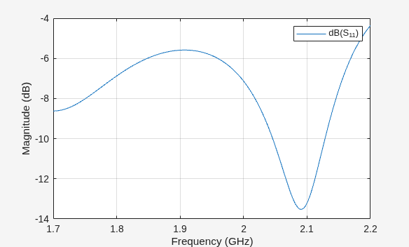
Use the sparameters function to calculate the $S_{11}$ of the helix antenna. Antenna reflection coefficient, or $S_{11}$ , describes a relative fraction of the incident RF power that is reflected back due to the impedance mismatch.

S = sparameters(hx,1.7e9:1e6:2.2e9,72)

S = 
  sparameters with properties:

      Impedance: 72
       NumPorts: 1
     Parameters: [1×1×501 double]
    Frequencies: [501×1 double]

rfplot(S)

$Figure contains an axes object. The axes object with xlabel Frequency (GHz), ylabel Magnitude (dB) contains an object of type line. This object represents dB(S_{11}).$

Calculate Return Loss

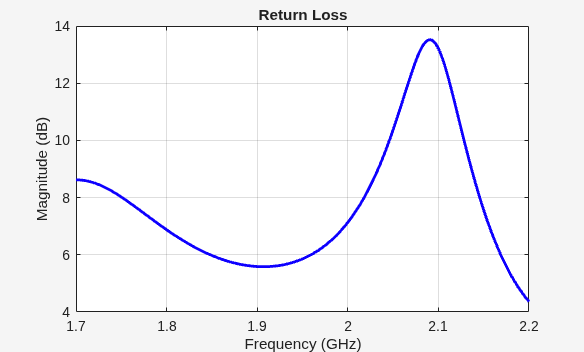
Use the returnLoss function to calculate and plot the return loss of the helix antenna. Antenna return loss is a measure of the effectiveness of power delivery from a transmission line to a load such as antenna. The calculations are displayed in log scale.

returnLoss(hx,1.7e9:1e6:2.2e9,72)

Figure contains an axes object. The axes object with title Return Loss, xlabel Frequency (GHz), ylabel Magnitude (dB) contains an object of type line.

Calculate Voltage Standing Wave Ratio (VSWR)

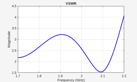
Use the vswr function to calculate and plot the VSWR of the helix antenna. The antenna VSWR is another measure of impedance matching between transmission line and antenna.

vswr(hx,1.7e9:1e6:2.2e9,72)

Figure contains an axes object. The axes object with title VSWR, xlabel Frequency (GHz), ylabel Magnitude contains an object of type line.

Calculate Current and Charge Distribution

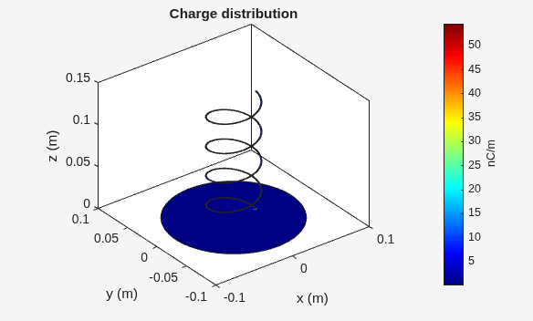
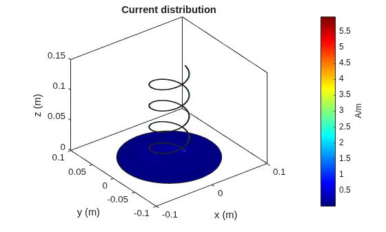
Use the charge function to calculate the charge distribution of the helix antenna. Charge distribution is the value of charge on the antenna surface at a specified frequency. Use the current function to calculate the current distribution of the helix antenna. Current distribution is the value of current on the antenna surface at a specified frequency.

charge(hx,2.01e9)

Figure contains an axes object. The axes object with title Charge distribution, xlabel x (m), ylabel y (m) contains 4 objects of type patch.

figure
current(hx,2.01e9)

Figure contains an axes object. The axes object with title Current distribution, xlabel x (m), ylabel y (m) contains 4 objects of type patch.

Create and Visualize Antenna Mesh

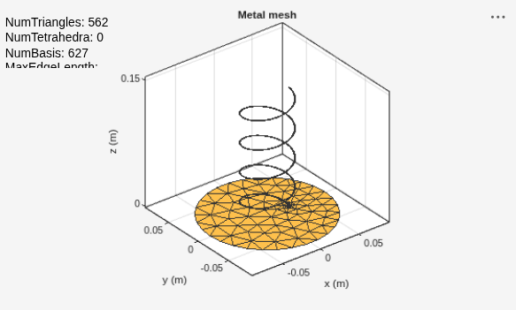
Use the mesh function to create and visualize a mesh structure for the helix antenna. Mesh is used to discretize antenna surface. In this process, the electromagnetic solver can process the geometry and material of the antenna. The shape of the basis or the discretizing element for subdividing the antenna surface is a triangle.

figure
mesh(hx)

Figure contains an axes object and an object of type uicontrol. The axes object with title Metal mesh, xlabel x (m), ylabel y (m) contains 2 objects of type patch, surface. These objects represent PEC, feed.

Mesh Antenna Manually

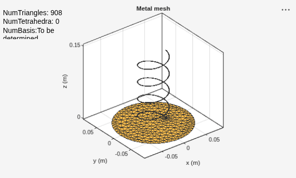
Specify the maximum edge length for the triangles using the MaxEdgeLength name-value argument. This meshes the helix structure manually.

figure
mesh(hx, MaxEdgeLength=0.01)

Change Mesh Mode to Automatic

Use the meshconfig function to change the mesh mode to automatic.

meshconfig(hx,"auto")

ans = struct with fields:
     NumTriangles: 908
    NumTetrahedra: 0
         NumBasis: []
    MaxEdgeLength: 0.0100
    MinEdgeLength: 0.0075
       GrowthRate: 0.9500
         MeshMode: 'auto'

References

[1] Balanis, Constantine A. Antenna Theory: Analysis and Design. 3rd ed. p. 514, John Wiley & Sons, New York, 2005.