Signal Recovery with Differentiable Scalograms and Spectrograms

R2026b

Since R2022b

This example demonstrates a gradient-descent-based phase-retrieval technique using differentiable spectrograms and scalograms. The example applies the gradient-descent-based technique to both synthetic and speech signals and compares the differentiable technique with the Griffin-Lim algorithm.

In a number of applications, the phase information in a time-frequency representation is discarded in favor of the magnitudes. There are a number of reasons for this. One reason is simply that the complex-valued time-frequency representations containing phase information are difficult to plot and interpret. This may lead people to retain only the magnitudes. In other applications, the required signal processing is optimally done by modifying the magnitudes of a time-frequency representation. This is most frequently done in speech processing where the underlying time-frequency representation is usually the short-time Fourier transform. In the latter case, the original complex-valued time-frequency representation no longer corresponds to the modified magnitude representation.

In these applications, it still may be useful or even necessary to recover an approximation of the original signal. The techniques for doing this are referred to as phase retrieval. Phase retrieval is, in general, ill-posed and prior iterative methods suffer from the non-convexity of the formulation and therefore convergence to an optimal solution is impossible to guarantee.

The incorporation of automatic differentiation and differentiable signal processing makes it feasible to perform gradient-descent phase retrieval with the usual convex loss functions. To recover a signal from the magnitude of its spectrogram, use stftmag2sig (Signal Processing Toolbox). To recover a signal from the magnitude of its scalogram, use cwtmag2sig. You must have a Deep Learning Toolbox™ license to use the gradient-descent algorithm.

Synthetic Signal — Exponential Chirp

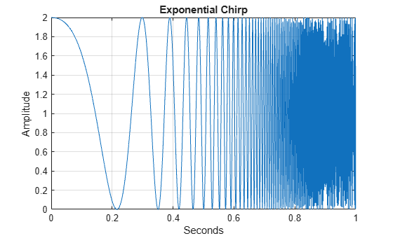
First, create a chirp signal with an exponentially increasing carrier frequency. This synthetic signal is challenging for a signal recovery, or phase retrieval, algorithm because the instantaneous frequency increases rapidly.

rng("default")
N = 2048;
fs = N;
a = 1;
b = fs/2;
t = (0:N-1)'/fs;
sig = chirp(t,a,t(end),b,"logarithmic") + 1;
plot(t,sig)
grid on
title("Exponential Chirp")
xlabel("Seconds")
ylabel("Amplitude")

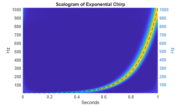
Obtain the scalogram of the chirp and plot the scalogram along with the instantaneous frequency of the chirp. Plot the scalogram using a linear scaling on the frequency (scale) axis to clearly show the exponential nature of the chirp.

[fmin,fmax] = cwtfreqbounds(2048,fs,Cutoff=100,wavelet="amor");
[cfs,f,~,~,scalcfs] = cwt( ...
    sig,fs,FrequencyLimits=[fmin fmax],Boundary="periodic");
t = linspace(0,1,length(sig));
surf(t,f,abs(cfs))
ylabel("Hz")
shading interp
view(0,90)
yyaxis right
plot(t,1024.^t,"k--")
axis tight
title("Scalogram of Exponential Chirp")
ylabel("Hz")
xlabel("Seconds")

Now, use a differentiable scalogram to perform phase retrieval. This examples uses the helper object, helperPhaseRetrieval, to perform phase retrieval for both the scalogram and spectrogram. By default, helperPhaseRetrieval pads the signal symmetrically with 10 samples at the beginning and 10 samples at the end to compensate for edge effects.

First, create an object configured for the scalogram and obtain the scalogram of the chirp signal. Confirm the scalogram contains only real-valued data.

pr = helperPhaseRetrieval( ...
    Method="scalogram",wavelet="morse",IncludeLowpass=true);
sc = obtainTFR(pr,sig);
isreal(sc)

ans = logical
   1

The scalogram is also a dlarray object, which allows you to record operations performed on it for automatic differentiation.

Signal Recovery Using Gradient Descent

Here we recover an approximation to the original signal using the magnitude scalogram and gradient descent. The helper function retrievePhase does this by the following procedure:

1. Generate a white-noise signal with the same length as the padded input signal.

2. Obtain the scalogram of the noise. Measure the mean squared error (MSE) between the scalogram of the target signal and the scalogram of the noise.

3. Use gradient descent with an Adam optimizer to update the noise signal based on the MSE loss between the target scalogram and the scalogram of the noise.

This procedure is detailed in [1]. At the end of the gradient-descent procedure, determine how the noise has converged to a reconstruction of the original signal.

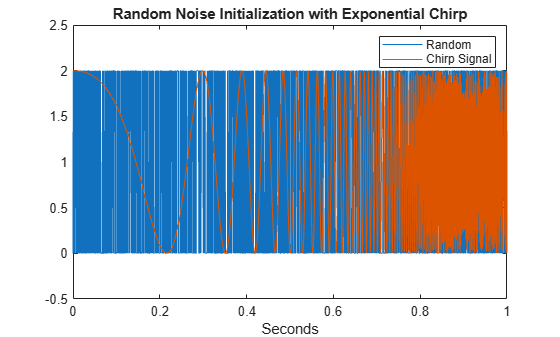
retrievePhase starts by creating a noise signal as a starting point. The following plot shows a representative noise that initiates the

gradient- descent procedure. Compare the initial noise signal with the original chirp signal.

rng("default")
x = dlarray(randn(length(sig)+20,1),"CBT");
xinit = x./max(abs(x),[],3)+1;
figure
plot(t,squeeze(extractdata(xinit(11:end-10,:,:))),LineWidth=0.5)
hold on
plot(t,sig)
legend(["Random" "Chirp Signal"])
title("Random Noise Initialization with Exponential Chirp")
axis tight
hold off
ylim([-0.5 2.5])
xlabel("Seconds")

Use gradient descent and the differentiable scalogram to recover an approximation to the original signal.

xrec = retrievePhase(pr,sc,InitialSignal=xinit);

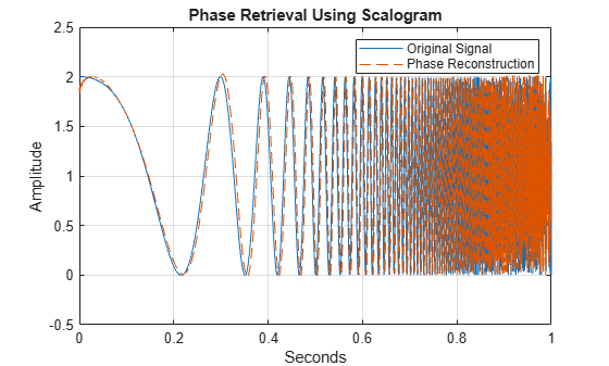
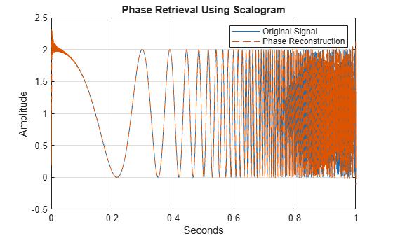
After 300 iterations of gradient descent, the noise signal is modified to closely approximate the chirp signal. Plot the result of the phase retrieval. Note that phase retrieval for real-valued signals is defined only up to a sign change. Accordingly, the result scaled by 1 or -1 may provide a better result.

plot(t,sig,t,xrec,"--")
grid on
xlabel("Seconds")
ylabel("Amplitude")
legend(["Original Signal" "Phase Reconstruction"])
title("Phase Retrieval Using Scalogram")

Repeat the computation using the cwtmag2sig function. For more information, see the function reference page.

xrec = cwtmag2sig(abs(cfs),fs,FrequencyLimits=[fmin fmax], ...
    ScalingCoefficients=scalcfs,Display=true);

#Iteration  |  Normalized Inconsistency  
      1     |  1.3560e+00 
     20     |  5.3378e-02 
     40     |  1.5615e-02 
     60     |  9.3957e-03 
     80     |  4.1989e-03 
    100     |  1.4131e-02 
    120     |  5.8552e-03 
    140     |  4.4652e-04 
    160     |  1.0685e-03 
    180     |  2.3087e-03 
    200     |  5.9261e-04 
    220     |  5.8277e-04 
    240     |  3.6967e-05 
    260     |  1.3581e-05 
    276     |  6.4125e-06 

Decomposition process stopped.
The normalized inconsistency for each channel is smaller than the "InconsistencyTolerance" of 1e-05.

plot(t,sig,t,xrec,"--")
grid on
xlabel("Seconds")
ylabel("Amplitude")
legend(["Original Signal" "Phase Reconstruction"])
title("Phase Retrieval Using Scalogram")

Obtain the scalogram of the reconstructed signal and compare its phase at selected center frequencies (CF) with the phase of the original. Compare the phase by plotting the real and imaginary parts of the continuous wavelet transform (CWT) coefficients separately.

cfsR = cwt(xrec,fs,FrequencyLimits=[fmin fmax]);
tiledlayout(3,2)
indices = [30 40 50];
xlimits = [0.63 0.79; 0.48 0.76; 0.4 0.62];

for i = 1:length(indices)
    idx = indices(i);
    fstr = sprintf("%2.2f",f(idx));

    nexttile(2*i-1)
    plot(t,real(cfs(idx,:))',t,real(cfsR(idx,:))',"--")
    grid on
    title("Scalogram (Real Part)", "CF " + fstr + " Hz")
    xlim(xlimits(i,:))
    
    nexttile(2*i)
    plot(t,imag(cfs(idx,:))',t,imag(cfsR(idx,:))',"--")
    grid on
    title("Scalogram (Imaginary Part)"," CF " + fstr + " Hz")
    xlim(xlimits(i,:))
end

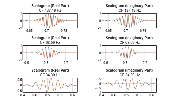
The phase agreement for the selected center frequencies is quite good. In fact, the wavelet coherence between the original signal and its reconstructed version using the gradient-descent approach is quite strong.

figure
wcoherence(sig,xrec,fs, ...
    FrequencyLimits=[0 1/2]*fs,PhaseDisplayThreshold=0.7)
title("Wavelet Coherence (Exponential Chirp with Reconstruction)", ...
    "Differentiable Scalogram with Gradient Descent");

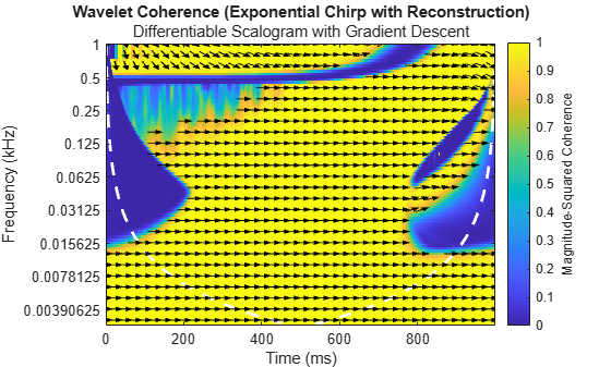
Repeat the same process using the spectrogram as the time-frequency representation instead of the scalogram. Evaluate the discrete Fourier transform at 128 points. Use the default settings for the stft function.

nfft = 128;
sp = stft(sig,FFTLength=nfft);
xrecGD = stftmag2sig(abs(sp),nfft, ...
    Method="gd",MaxIterations=600);

plot(t,sig,t,xrecGD,"--")
grid on
legend(["Original Signal" "Phase Reconstruction"])
title("Phase Retrieval (Gradient Descent)")
axis padded

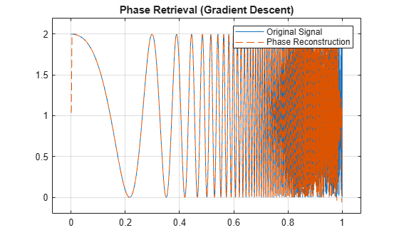
The recovery from the spectrogram is also quite good. Use wavelet coherence again to look at the time-varying phase coherence between the original signal and the output of phase-retrieval approach using gradient descent with the differentiable spectrogram.

wcoherence(sig,xrecGD,fs, ...
    FrequencyLimits=[0 1/2]*fs,PhaseDisplayThreshold=0.7)
title("Wavelet Coherence (Exponential Chirp with Reconstruction)", ...
    "Differentiable Spectrogram with Gradient Descent")

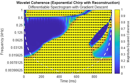
The phase coherence between the two signals is strong except at the start and finish of the signal in the high-frequency range.

The spectrogram plot shows that the frequency content of the original signal is concentrated at the low and high ends of the frequency range, respectively, so you have to be careful when interpreting the results. Meanwhile, in the area where the signal is primarily distributed, the phase coherence in the corresponding part of the wavelet coherence diagram is very strong.

figure(Position=[0 0 1500 600])
tiledlayout(1,2)
nexttile
stft(sig,fs,FFTLength=nfft,FrequencyRange="onesided")
set(gca,YScale="log");
title("Spectrogram of the Original Signal")
nexttile
wcoherence(sig,xrecGD, ...
    fs,FrequencyLimits=[0 1/2]*fs,PhaseDisplayThreshold=0.7)

Comparison with Griffin-Lim

Repeat the computation using the Griffin-Lim algorithm. The Griffin-Lim procedure requires the inverse short-time Fourier transform at every iteration and exhibits edge effects.

S = stft(sig);
xrecGL = stftmag2sig(abs(sp),nfft, ...
    Method="gl",MaxIterations=600);

figure
plot(t,sig,t,xrecGL,"--")
grid on
legend(["Original Signal" "Phase Reconstruction"])
title("Phase Retrieval (Griffin-Lim)")

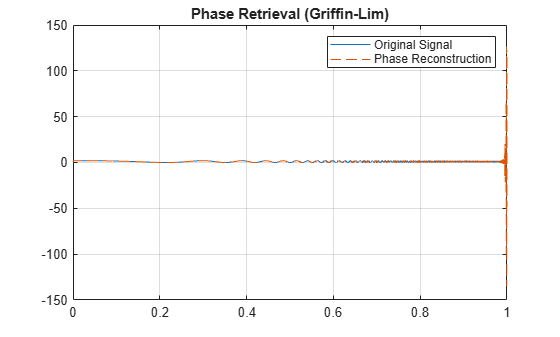
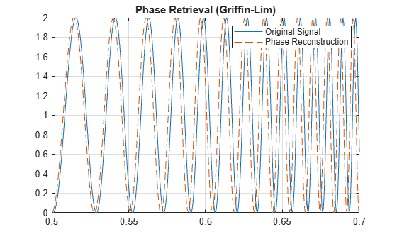
As anticipated, Griffin-Lim exhibits substantial deviation at the end of the signal. Moreover, upon closer observation, it can be noticed that in this case, it also presents significant discrepancy in the reconstruction of the signal's middle section.

plot(t,sig,t,xrecGL,"--")
ylim([0,2])
xlim([0.5 0.7])
grid on
legend(["Original Signal" "Phase Reconstruction"])
title("Phase Retrieval (Griffin-Lim)")

Use the original reconstruction from the STFT magnitudes using the Griffin-Lim algorithm and examine the wavelet coherence between the original signal and the reconstruction.

wcoherence(sig,xrecGL,fs, ...
    FrequencyLimits=[0 1/2]*fs,PhaseDisplayThreshold=0.7)
title("Wavelet Coherence (Exponential Chirp with Reconstruction)", ...
    "Griffin-Lim Algorithm using Spectrograms")

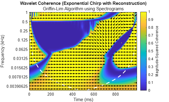
The Griffin-Lim algorithm is less accurate than the gradient-descent method in the high-frequency areas where the signal primarily resides.

In this instance, the differentiable phase-retrieval technique does a significantly better job at reconstructing the original phase than the Griffin-Lim algorithm. You can verify this numerically by examining the relative L2-norm error between the original signal and the approximations.

RelativeL2DiffGD = norm(sig-xrecGD,2)/norm(sig,2)

RelativeL2DiffGD = 
0.1075

RelativeL2DiffGL = norm(sig-xrecGL,2)/norm(sig,2)

RelativeL2DiffGL = 
4.5252

Speech Signal

A common application of signal recovery from magnitude time-frequency transforms is in speech.

Load and play a speech sample of a speaker saying "I saw the sheep". The original data is sampled at 22050 Hz, resample the data at 1/2 the original rate.

load wavsheep.mat
xsheep = resample(sheep,1,2);
fs = fs/2;
soundsc(xsheep,fs)
t = 0:1/fs:(length(xsheep)-1)/fs;

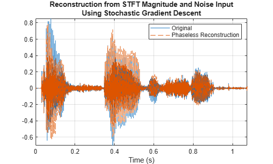
Recover an approximation of the speech signal from the magnitude spectrogram using gradient descent. Use a Hamming window with 256 samples and overlap the windows by 75% of the window length or 192 samples. Use 200 iterations of gradient descent and a different optimizer, the limited-memory Broyden–Fletcher–Goldfarb–Shanno (L-BFGS) optimizer, which usually gives better results at the cost of longer computation time.

win = hamming(256);
overlap = 0.75*256;
scsheep = stft(xsheep,Window=win,OverlapLength=overlap);

xrecGDsheep = stftmag2sig( ...
    abs(scsheep),length(win),Window=win,OverlapLength=overlap, ...
    Method="gd",Optimizer="lbfgs",MaxIterations=300);

The reconstructed signal is very similar to the original. The π/2 ambiguity that inverts some peaks is expected and does not affect the perceived sound.

idx = 1:length(xrecGDsheep);

plot(t(idx),xsheep(idx),t(idx),xrecGDsheep,"--")
title(["Reconstruction from STFT Magnitude and Noise Input", ...
    "Using Stochastic Gradient Descent"])
legend("Original","Phaseless Reconstruction")
xlabel("Time (s)")
axis tight
grid on

Play the original waveform and the reconstruction. Pause 3 seconds between playbacks.

soundsc(xsheep,fs)
pause(3)
soundsc(xrecGDsheep,fs)

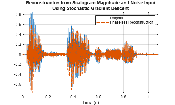
Repeat the procedure using as input the magnitude of the CWT. The CWT is more computationally expensive than the STFT and takes longer to compute. Accelerate the computation using a graphical processing unit (GPU), if available. To determine the reduction in computation time, toggle back and forth between the true and false options.

useGPU = false;
[fmin,fmax] = cwtfreqbounds(2048,Cutoff=100,wavelet="amor");
[cfs,~,~,~,scalcfs] = cwt(xsheep, ...
    FrequencyLimits=[fmin fmax],Boundary="periodic");

if useGPU
    cfs = gpuArray(cfs); %#ok<UNRCH>
end
xrecGDsheep = cwtmag2sig(abs(cfs),FrequencyLimits=[fmin fmax], ...
    ScalingCoefficients=scalcfs,Optimizer="sgdm");

Plot the result. Similar to the case with the magnitude STFT, what began as random noise has converged to a good approximation of the speech signal. There is always a phase ambiguity between a value V and its negative -V. So you can also plot result scaled by -1.

plot(t,xsheep,t,xrecGDsheep,"--")
title(["Reconstruction from Scalogram Magnitude and Noise Input", ...
    "Using Stochastic Gradient Descent"])
legend(["Original" "Phaseless Reconstruction"])
xlabel("Time (s)")
axis tight
grid on

Play the original waveform and the reconstruction. Pause 3 seconds between playbacks. The scalogram technique also produces an approximation that is perceptually equivalent to the original.

soundsc(xsheep,fs)
pause(3)
soundsc(xrecGDsheep,fs)

Conclusion

This example demonstrates the algorithms and functions that employ differentiable signal processing and gradient descent to recover signal approximations from magnitude time-frequency representations. The approach has many advantages over traditional iterative methods based on inverse transform like the Griffin-Lim algorithm. For instance, it is less affected by minor edge effects and, in many cases, provides superior signal recovery. It allows for targeted selection among various optimizers and benefits from GPU acceleration. Furthermore, this method does not depend on the implementation of an inverse transform, making it easily expandable.