Main Content

wvd

Wigner-Ville distribution and smoothed pseudo Wigner-Ville distribution

Description

example

d = wvd(x) returns the Wigner-Ville distribution of x.

example

d = wvd(x,fs) returns the Wigner-Ville distribution when x is sampled at a rate fs.

example

d = wvd(x,ts) returns the Wigner-Ville distribution when x is sampled with a time interval ts between samples.

d = wvd(___,"smoothedPseudo") returns the smoothed pseudo Wigner-Ville distribution of x. The function uses the length of the input signal to choose the lengths of the windows used for time and frequency smoothing. This syntax can include any combination of input arguments from previous syntaxes.

example

d = wvd(___,"smoothedPseudo",twin,fwin) specifies the time window, twin, and the frequency window, fwin, used for smoothing. To use the default window for either time or frequency smoothing, specify the corresponding argument as empty, [].

example

d = wvd(___,"smoothedPseudo",Name=Value) specifies additional options for the smoothed pseudo Wigner-Ville distribution using name-value arguments. You can specify twin and fwin in this syntax, or you can omit them.

example

d = wvd(___,MinThreshold=thresh) sets to zero those elements of d whose amplitude is less than thresh. This syntax applies to both the Wigner-Ville distribution and the smoothed pseudo Wigner-Ville distribution.

example

[d,f,t] = wvd(___) also returns a vector of frequencies f and a vector of times t at which d is computed.

wvd(___) with no output arguments plots the Wigner-Ville or smoothed pseudo Wigner-Ville distribution in the current figure.

Examples

collapse all

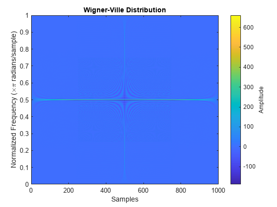
Generate a 1000-sample impulse and a 1000-sample tone with normalized frequency π/2. Compute the Wigner-Ville distribution of the sum of the two signals.

x = zeros(1001,1);
x(500) = 10;

y = sin(pi*(0:1000)/2)';

[d,f,t] = wvd(x+y);

Plot the Wigner-Ville distribution.

imagesc(t,f,d)
axis xy
colorbar

Reproduce the result by calling wvd with no output arguments.

wvd(x+y)

Generate a signal consisting of a 200 Hz sinusoid sampled at 1 kHz for 1.5 seconds.

fs = 1000;
t = (0:1/fs:1.5)';
x = cos(2*pi*t*200);

Compute the Wigner-Ville distribution of the signal.

wvd(x,fs)

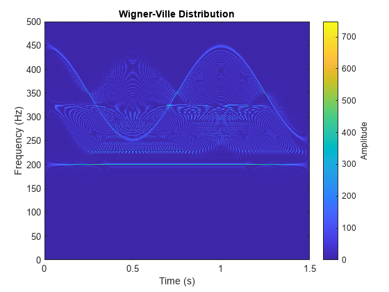
Add to the signal a chirp whose frequency varies sinusoidally between 250 Hz and 450 Hz. Convert the signal to a MATLAB® timetable. Compute the Wigner-Ville distribution.

x = x + vco(cos(2*pi*t),[250 450],fs);
xt = timetable(seconds(t),x);

wvd(xt)

Set to zero the distribution elements with amplitude less than 0.

wvd(xt,MinThreshold=0)

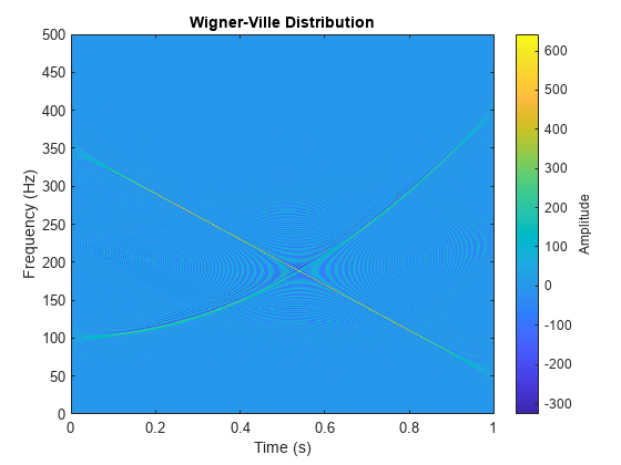
Generate a signal sampled at 1 kHz for 1 second. One component of the signal is a chirp that increases in frequency quadratically from 100 Hz to 400 Hz during the measurement. The other component of the signal is a chirp that decreases in frequency linearly from 350 Hz to 50 Hz in the same lapse.

Store the signal in a timetable.

fs = 1000;
t = 0:1/fs:1;

x = chirp(t,100,1,400,"quadratic") + chirp(t,350,1,50);

Compute the Wigner-Ville distribution of the signal.

wvd(x,fs)

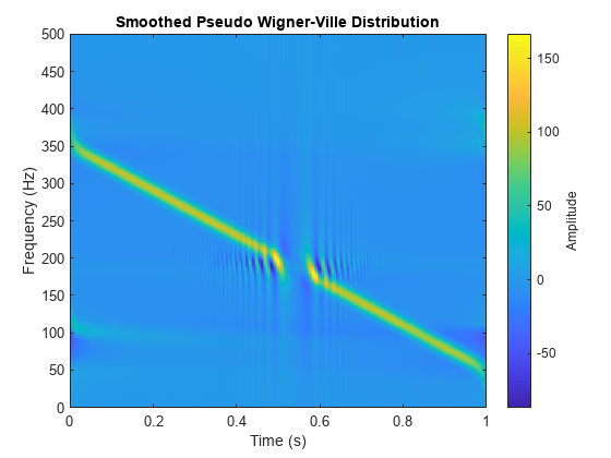
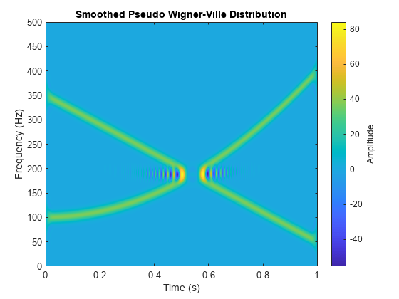
Compute the smoothed pseudo Wigner-Ville distribution of the signal. Specify 501 frequency points and 502 time points.

wvd(x,fs,"smoothedPseudo",NumFrequencyPoints=501,NumTimePoints=502)

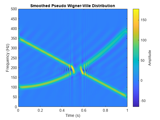
Increase the number of time points so the quadratic chirp becomes visible.

wvd(x,fs,"smoothedPseudo",NumFrequencyPoints=501,NumTimePoints=522)

Increase the frequency points and time points to get a sharper image.

wvd(x,fs,"smoothedPseudo",NumFrequencyPoints=1000,NumTimePoints=1502)

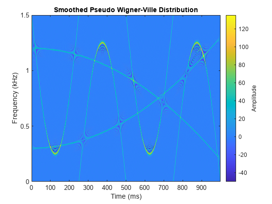
Generate a two-component signal sampled at 3 kHz for 1 second. The first component is a quadratic chirp whose frequency increases from 300 Hz to 1300 Hz during the measurement. The second component is a chirp with sinusoidally varying frequency content. The signal is embedded in white Gaussian noise. Express the time between consecutive samples as a duration scalar.

fs = 3000;
t = 0:1/fs:1-1/fs;
dt = seconds(t(2)-t(1));

x1 = chirp(t,300,t(end),1300,"quadratic");
x2 = exp(2j*pi*100*cos(2*pi*2*t));

x = x1 + x2 + randn(size(t))/10;

Compute and plot the smoothed pseudo Wigner Ville of the signal. Window the distribution in time using a 601-sample Hamming window and in frequency using a 305-sample rectangular window. Use 600 frequency points for the display. Set to zero those components of the distribution with amplitude less than -50.

wvd(x,dt,"smoothedPseudo",hamming(601),rectwin(305), ...
    NumFrequencyPoints=600,MinThreshold=-50)

Generate a signal composed of four Gaussian atoms. Each atom consists of a sinusoid modulated by a Gaussian. The sinusoids have frequencies of 100 Hz and 400 Hz. The Gaussians are centered at 150 milliseconds and 350 milliseconds and have a variance of 0.012. All atoms have unit amplitude. The signal is sampled at 1 kHz for half a second.

fs = 1000;
t = (0:1/fs:0.5)';

f1 = 100;
f2 = 400;

mu1 = 0.15;
mu2 = 0.35;

gaussFun = @(A,x,mu,f) exp(-(x-mu).^2/(2*0.01^2)).*sin(2*pi*f.*x)*A';

s = gaussFun([1 1 1 1],t,[mu1 mu1 mu2 mu2],[f1 f2 f1 f2]);

Compute and display the Wigner-Ville distribution of the signal. Interference terms, which can have negative values, appear halfway between each pair of auto-terms.

wvd(s,fs)

Compute and display the smoothed pseudo Wigner-Ville distribution of the signal. Smoothing in time and frequency attenuates the interference terms.

wvd(s,fs,"smoothedPseudo")

Input Arguments

collapse all

Input signal, specified as a vector or a MATLAB® timetable containing a single vector variable.

If the input signal has odd length, the function appends a zero to make the length even.

Example: cos(pi/8*(0:159))'+randn(160,1)/10 specifies a sinusoid embedded in white noise.

Example: timetable(seconds(0:5)',rand(6,1)) specifies a random variable sampled at 1 Hz for 5 seconds.

Data Types: single | double
Complex Number Support: Yes

Sample rate, specified as a positive numeric scalar.

Sample time, specified as a duration scalar.

Time and frequency windows used for smoothing, specified as vectors of odd length. By default, wvd uses Kaiser windows with shape factor β = 20.

  • The default length of twin is the smallest odd integer greater than or equal to round(length(x)/10).

  • The default length of fwin is the smallest odd integer greater than or equal to nf/4, where nf is specified using NumFrequencyPoints.

Each window must have a length smaller than or equal to 2*ceil(length(x)/2).

Example: kaiser(65,0.5) specifies a 65-sample Kaiser window with a shape factor of 0.5.

Minimum nonzero value, specified as a real scalar. The function sets to zero those elements of d whose amplitudes are less than thresh.

Name-Value Arguments

Specify optional pairs of arguments as Name1=Value1,...,NameN=ValueN, where Name is the argument name and Value is the corresponding value. Name-value arguments must appear after other arguments, but the order of the pairs does not matter.

Before R2021a, use commas to separate each name and value, and enclose Name in quotes.

Example: 'NumFrequencyPoints',201,'NumTimePoints',300 computes the Wigner-Ville distribution at 201 frequency points and 300 time points.

Number of frequency points, specified as an integer. This argument controls the degree of oversampling in frequency. The number of frequency points must be at least (length(fwin)+1)/2 and cannot be greater than the default.

Number of time points, specified as an even integer. This argument controls the degree of oversampling in time [3] (Signal Processing Toolbox). The number of time points must be at least 2*length(twin) and cannot be greater than the default.

Tip

If the input signal is large, reduce the number of time points to lower the memory requirements and speed up the computation.

Output Arguments

collapse all

Wigner-Ville distribution, returned as a matrix. Time increases across the columns of d, and frequency increases down the rows. The matrix is of size Nf × Nt, where Nf is the length of f and Nt is the length of t.

Frequencies, returned as a vector.

  • If the input has time information, then f contains frequencies expressed in Hz.

  • If the input does not have time information, then f contains normalized frequencies expressed in rad/sample.

Time instants, returned as a vector.

  • If the input has time information, then t contains time values expressed in seconds.

  • If the input does not have time information, then t contains sample numbers.

More About

collapse all

Wigner-Ville Distribution

The Wigner-Ville distribution provides a high-resolution time-frequency representation of a signal. The distribution has applications in signal visualization, detection, and estimation.

For a continuous signal x(t), the Wigner-Ville distribution is defined as

WVDx(t,f)=x(t+τ2)x*(tτ2)ej2πfτdτ.

For a discrete signal with N samples, the distribution becomes

WVDx(n,k)=m=NNx(n+m/2)x*(nm/2)ej2πkm/N.

For odd values of m, the definition requires evaluation of the signal at half-integer sample values. It therefore requires interpolation, which makes it necessary to zero-pad the discrete Fourier transform to avoid aliasing.

The Wigner-Ville distribution contains interference terms that often complicate its interpretation. To sharpen the distribution, one can filter the definition with lowpass windows. The smoothed pseudo Wigner-Ville distribution uses independent windows to smooth in time and frequency:

SPWVDxg,H(t,f)=g(t)H(f)x(t+τ2)x*(tτ2)ej2πfτdτ.

References

[1] Cohen, Leon. Time-Frequency Analysis: Theory and Applications. Englewood Cliffs, NJ: Prentice-Hall, 1995.

[2] Mallat, Stéphane. A Wavelet Tour of Signal Processing. Second Edition. San Diego, CA: Academic Press, 1999.

[3] O'Toole, John M., and Boualem Boashash. "Fast and Memory-Efficient algorithms for Computing Quadratic Time-Frequency Distributions." Applied and Computational Harmonic Analysis. Vol. 35, Number 2, 2013, pp. 350–358.

Extended Capabilities

C/C++ Code Generation
Generate C and C++ code using MATLAB® Coder™.

GPU Code Generation
Generate CUDA® code for NVIDIA® GPUs using GPU Coder™.

Version History

Introduced in R2018b

expand all

See Also

Functions