Die Übersetzung dieser Seite ist veraltet. Klicken Sie hier, um die neueste Version auf Englisch zu sehen.

Kontinuierliche Wavelet-Transformation und inverse kontinuierliche Wavelet-Transformation

Dieses Beispiel zeigt die Verwendung der kontinuierlichen Wavelet-Transformation (Continuous Wavelet Transform, CWT) und der inversen CWT.

CWT von Sinuswellen und Impulsen

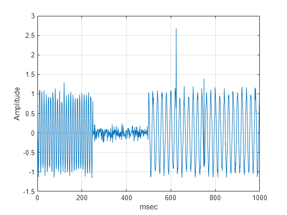
Konstruieren und plotten Sie ein Signal aus zwei disjunkten Sinuswellen mit Frequenzen von 100 und 50 Hz, in denen zwei Impulse auftreten. Die Abtastfrequenz beträgt 1 kHz und die Gesamtsignaldauer eine Sekunde. Die 100-Hz-Sinuswelle tritt in den ersten 250 Millisekunden der Daten auf. Die 50-Hz-Sinuskurve tritt in den letzten 500 Millisekunden auf. Die Impulse treten bei 650 und 750 Millisekunden auf. Das Signal weist außerdem ein additives weißes Gauß‘sches Rauschen von $N (0, 0.1^{2})$ auf. Der Impuls bei 650 Millisekunden ist sichtbar, der Impuls bei 750 Millisekunden ist jedoch in den Zeitbereichsdaten nicht klar ersichtlich.

Fs = 1000;
t = 0:1/Fs:1-1/Fs;
x = zeros(size(t));
x([625,750]) = 2.5;
x = x+ cos(2*pi*100*t).*(t<0.25)+cos(2*pi*50*t).*(t>=0.5)+...
    0.1*randn(size(t));
plot(t.*1000,x)
grid on;
xlabel('msec'); ylabel('Amplitude');

Figure contains an axes object. The axes object with xlabel msec, ylabel Amplitude contains an object of type line.

Ermitteln und plotten Sie die CWT mit dem standardmäßigen analytischen Morse-Wavelet.

[cfs,f] = cwt(x,1000);
contour(t.*1000,f,abs(cfs));
xlabel('msec'); ylabel('Hz');
grid on;

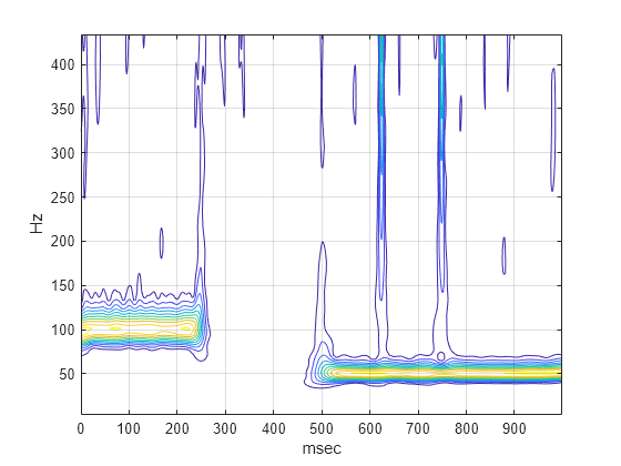
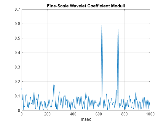
Figure contains an axes object. The axes object with xlabel msec, ylabel Hz contains an object of type contour.

Die CWT-Absolutwerte zeigen deutlich die Träger der disjunkten Sinuskurven und die Stellen der Impulse bei 650 und 750 Millisekunden. In den CWT-Absolutwerten ist der Impuls bei 750 Millisekunden deutlich sichtbar. Dies gilt insbesondere, wenn Sie nur die feinskaligsten Wavelet-Koeffizienten plotten.

plot(t.*1000,abs(cfs(1,:)))
grid on
title('Fine-Scale Wavelet Coefficient Moduli')
xlabel('msec')

Figure contains an axes object. The axes object with title Fine-Scale Wavelet Coefficient Moduli, xlabel msec contains an object of type line.

In Frequenz lokalisierte inverse CWT

Mit der inversen CWT können Sie in der Frequenz lokalisierte Approximationen für Ereignisse in Ihren Zeitreihen konstruieren. Verwenden Sie die inverse CWT, um eine Approximation an die 100-Hz-Sinuskurve im vorherigen Beispiel zu erhalten.

xrec = icwt(cfs,[],f,[90 110]);
plot(t,x);
hold on;
plot(t,xrec,'r');
legend('Original Signal','Inverse CWT Approximation',...
    'Location','NorthEast');
grid on;

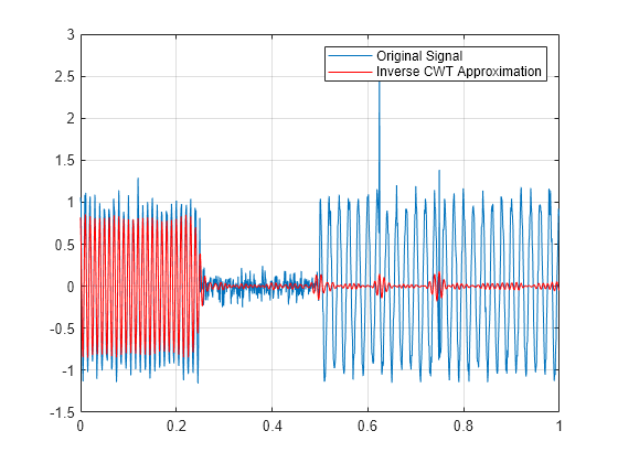
Figure contains an axes object. The axes object contains 2 objects of type line. These objects represent Original Signal, Inverse CWT Approximation.

Wenn Sie die Darstellung vergrößern, sehen Sie, dass die 100-Hz-Komponente gut approximiert wird, während die 50-Hz-Komponente entfernt wurde.