Video Stabilization
This example shows how to implement a feature-based video stabilization algorithm for FPGAs.
This algorithm helps reduce shaking between frames. Digital video stabilization techniques provide a more feasible and economical solution than a physical stabilizer.
This example implements the same algorithm as the Stabilize Video Using Image Point Features (Computer Vision Toolbox) example. The video stabilization algorithm has these steps.
Features from accelerated segment test (FAST) feature detector — Detect corners as features to match between the two frames.
Binary robust independent elementary features (BRIEF) descriptor — Calculate a unique description for each feature.
Feature matching — Match each feature description with its corresponding feature in the other frame.
Random sample consensus (RANSAC) affine transformation estimation — Calculate a transform that describes the movement of the second frame relative to the first one.
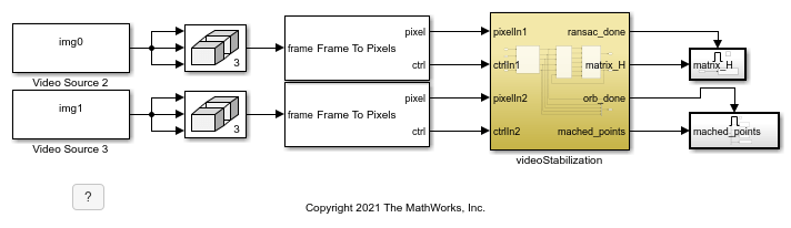
The videoStabilization subsystem has four output ports.
ransac_done indicates the completion of RANSAC.
matrix_H is the transform matrix in the form [[a, d, 0], [b, e, 0], [c, f, 1]].
orb_done indicates the ORB (oriented FAST rotated BRIEF) part is done.
matched_points is the matched points from ORB matching.
The last two output signals are for additional information or debugging.
modelname = 'VideoStabilizationHDL';
open_system(modelname);
set_param(modelname,'SampleTimeColors','on');
set_param(modelname,'Open','on');
set(allchild(0),'Visible','off');
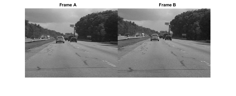
These images show consecutive frames from a camera.
imgA = imread('VideoStabilizationHDLExample_img_0.png');
imgB = imread('VideoStabilizationHDLExample_img_1.png');
figure; imshowpair(imgA, imgB, 'montage');
title(['Frame A', repmat(' ',[1 70]), 'Frame B']);
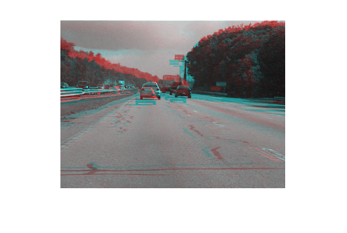
To highlight the difference, the figure shows a red-cyan color composite to show the pixel-wise difference between them. Frame A is shown in red, and frame B is shown in cyan.
figure; imshowpair(imgA,imgB,'ColorChannels','red-cyan');
FAST Feature Detection
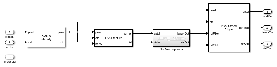
This part of the algorithm follows the design concept outlined in the FAST Corner Detection example to design a 9-16 FAST detector. The 9-16 FAST feature point detector finds the pixel value difference between the central pixel and its surrounding pixels, as shown in this figure.
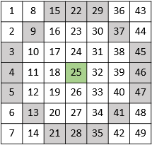
If 7 out of 12 pixels have a larger pixel value difference than a specified threshold, the detector considers the central point as a feature point. Then, the NonMaxSuppress subsystem filters out features that have less than the maximum metric within a 5-by-5 patch window. The figure shows the FAST subsystem.
open_system([modelname '/videoStabilization/oFAST_rBRIEF/FAST_1'],'force');
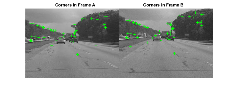
This figure shows the detected corners.
imgA_fast = imread('VideoStabilizationHDLExample_a_fast.png');
imgB_fast = imread('VideoStabilizationHDLExample_b_fast.png');
figure; imshowpair(imgA_fast, imgB_fast, 'montage');
title([ 'Corners in Frame A', repmat(' ',[1 40]),'Corners in Frame B']);
BRIEF Descriptor Generation
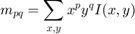
The purpose of a feature descriptor is to generate a unique string for each feature point. The algorithm uses these strings to match points between frames. The BRIEF descriptor generates a binary vector for each feature point returned from corner detection by comparing the pixel values in a fixed pattern [3]. This example uses oriented FAST features (oFAST) to increase robustness to image rotation. The oFAST algorithm rotates each image patch to align it to a common direction before generating its binary vector. The angle of rotation is the angle between the intensity centroids of both x-axis and y-axis, as defined by this equation.
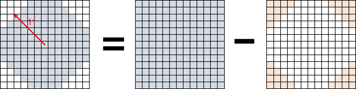
The algorithm calculates the intensity centroid by using a circular patch. In this case, the radius of the circle is 11. The algorithm calculates the weighted sum of a square patch and then subtracts the values at the corners. This figure shows the creation of a circular patch from a square patch.
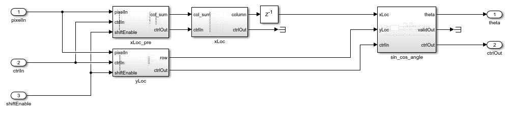
After intensity centroid calculation, the Complex to Magnitude-Angle (DSP HDL Toolbox) block computes the rotation angle. The figure shows the BRIEF descriptor generator.
open_system([modelname '/videoStabilization/oFAST_rBRIEF/BRIEF_DESC_GEN_1/IntensityCentroid'],'force');
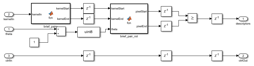
Before applying the fixed pattern, the BRIEF block rotates this circular patch by the computed angle. The fixed pattern used in this model comes from OpenCV software [3].
open_system([modelname '/videoStabilization/oFAST_rBRIEF/BRIEF_DESC_GEN_1/descriptor_gen'],'force');
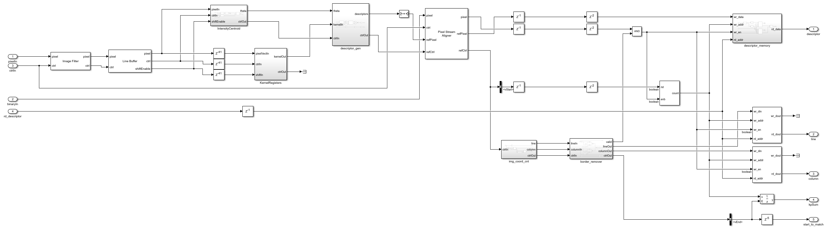
Because the BRIEF algorithm compares the pixel value of each fixed pair, the description generator is an array of comparators. The model stores the output binary vectors in the on-chip memory. The example supports 1024 features by default. You can change the number of features by setting the Estimated number of feature points parameter of the oFAST_rBRIEF subsystem. This parameter configures the size of the Simple Dual Port RAM blocks in the BRIEF_DESC_GEN_1 and descriptor_memory subsystems. This figure shows the BRIEF descriptor generation subsystem.
open_system([modelname '/videoStabilization/oFAST_rBRIEF/BRIEF_DESC_GEN_1'],'force');
Feature Matching
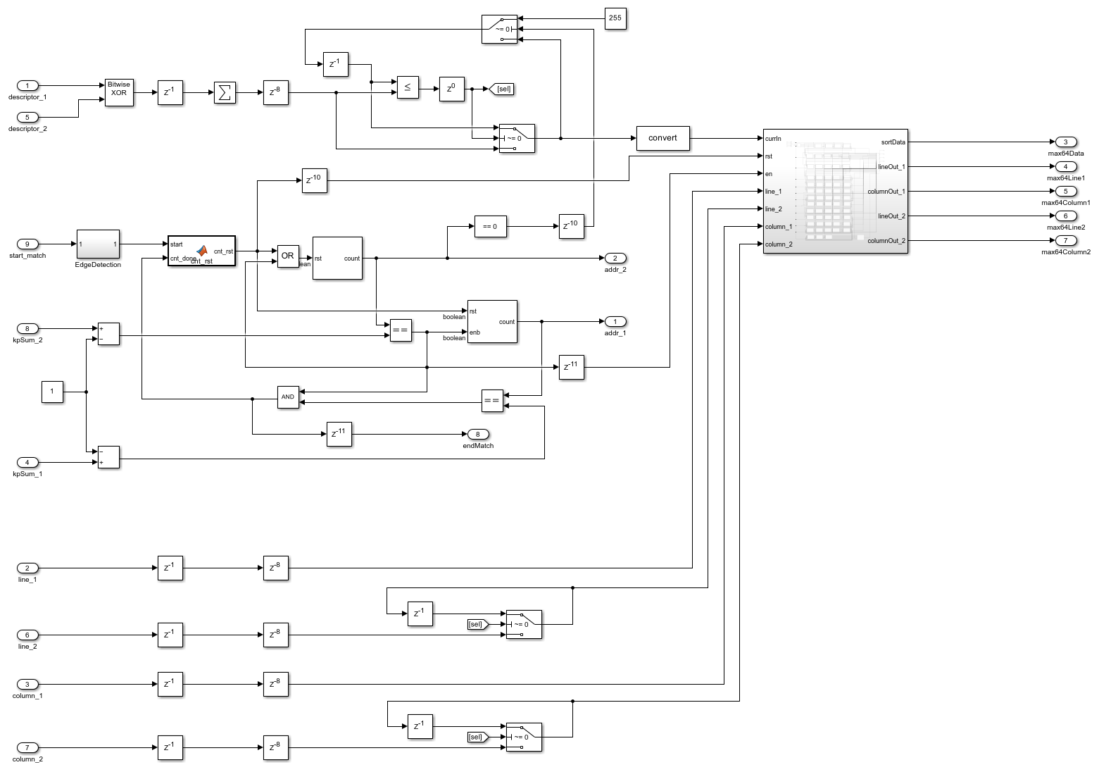
This figure shows the matching process that uses the binary BRIEF feature descriptors.
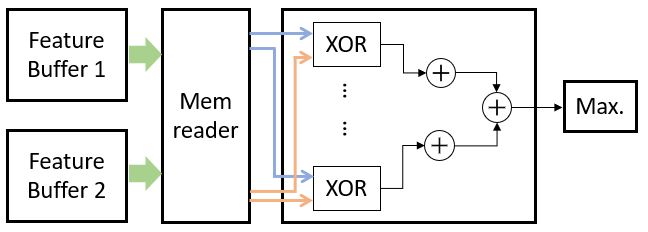
Because of the complexity of implementing sorting algorithms on hardware, this example implements a simple bubble-sorting algorithm to find the 64 best matched point pairs from two images. The bubble-sorting algorithm consumes fewer resources than a parallel sort. Because each image typically has hundreds of feature points, finding each pair of points would cost hundreds of clock cycles if you performed exhaustive matching. The time used by bubble sorting is much shorter than an exhaustive match.
open_system([modelname '/videoStabilization/oFAST_rBRIEF/BRIEF_MATCH'],'force');
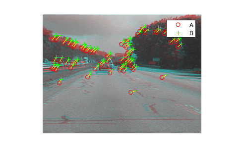
This image shows the results of matching feature points.
RANSAC Affine Transformation Estimation
RANSAC is a common algorithm for finding an optimal affine transform. The key idea of RANSAC is to repeatedly pick three random point pairs, and then calculate the affine transform matrix. The algorithm stops repeating when either 95% of the point pairs match (error is less than 2 pixels) or the algorithm completes the maximum number of iterations. You can change these parameters in the RANSAC subsystem mask.
open_system([modelname '/videoStabilization/RANSAC'],'force');
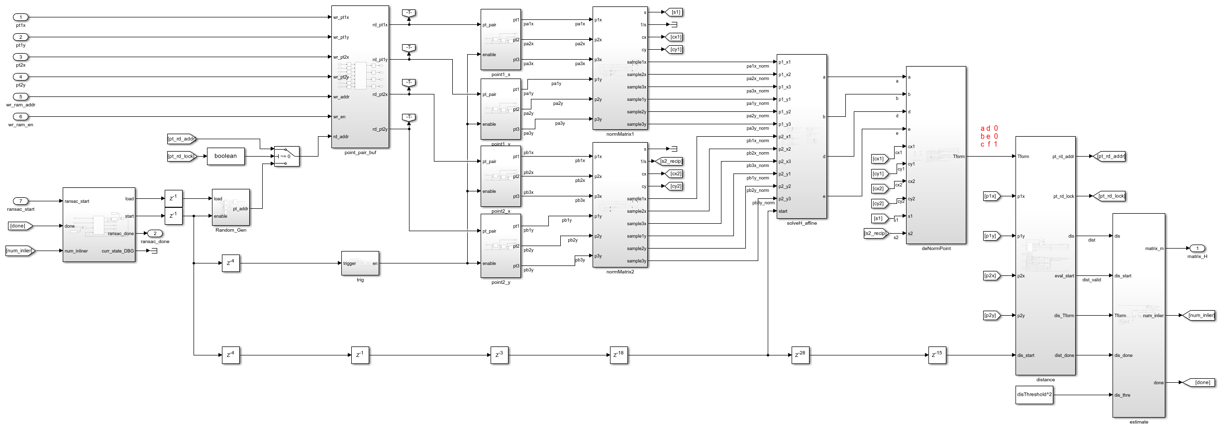
The standard procedure for RANSAC calculation comprises these steps.
Random selection — To reduce the computation burden of RANSAC, give the algorithm only the best matched 64 point pairs. The linear-feedback shift register (LFSR) randomly selects 3 of these 64 point pairs.
Normalization — Normalize point location (x,y) into 1.x format. This normalization is critical to guarantee a stable result from RANSAC.
Calculate affine matrix — Solve linear equations with six variables. This block implements the numerical solution of these equations. Because additional latency at this step does not affect the throughput of the design, this subsystem implements a fully pipelined simple divider. The simple divider uses fewer resources than other divider implementations for hardware. #Denormalization — Convert the point location back to (x,y) format. This operation is the inverse of normalization.
Model Configuration
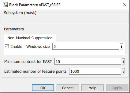
You can configure these parameters on the subsystems.
Nonmaximal suppression — To reduce processing of extra features, enable nonmaximal suppression. You can also select the patch size. Typical patch sizes are five or seven pixels. Larger patch sizes result in fewer features with low FAST scores, but longer latency.
Minimum contrast for FAST — The typical range for this threshold is 15 to 20, but the value varies for different applications.
Estimated number of feature points — This parameter determines the depth of on-chip memory. This parameter is defined by this equation.
 , where
  is the estimated number of features.
For example, the default value is 1000, which results in an on-chip memory depth of 1024 to store feature descriptors.
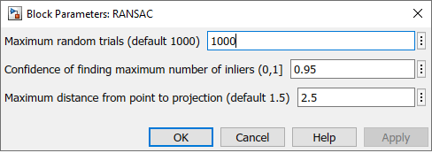
Maximum random trials — The default number of iterations is 1000. This value is usually less than 2000.
Confidence of finding maximum number of inliers — Percentage of point pairs matched. Because this algorithm uses only the 64 best-matched pairs, this example uses a confidence value of 95%. If your design uses more point pairs, you can reduce this parameter.
Maximum distance from point to projection — The recommended range of this parameter is from 1.5 to 2.
Performance
The figure shows the stabilization result obtained by applying the generated affine transform to the second input frame.
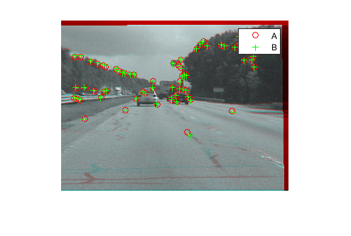
Because the camera is mounted on a moving vehicle, it has a different relative speed to the ground and to other vehicles on the road. Therefore, the matched point varies according to its position on the image. One way to extend this algorithm for applications with very large object size changes is to use an image pyramid to find features at different scales.
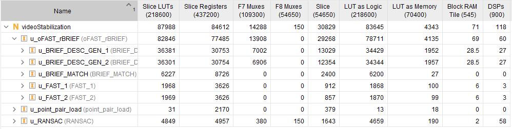
This design takes about 5 minutes to run an HDL simulation for 240p image/video with no more than 1024 feature points. This table shows the resource consumption on the AMD® Zynq®-7000 SoC ZC706 development kit.
References
[1] Rosten, E., and T. Drummond. "Fusing Points and Lines for High Performance Tracking." Proceedings of the IEEE International Conference on Computer Vision 2 (October 2005): 1508-1511.
[2] Rosten, E., and T. Drummond. "Machine Learning for High-Speed Corner Detection." Computer Vision - ECCV 2006 Lecture Notes in Computer Science (2006): 430-43. doi:10.1007/11744023_34.
[3] "OpenCV: Open Source Computer Vision Library" https://github.com/opencv/opencv, 2017
[4] Rublee, E., Rabaud, V., Konolige, K., and Bradski, G.. "ORB: An efficient alternative to SIFT or SURF." Proceedings of the IEEE International Conference on Computer Vision (2011): 2564-2571.
[5] Fischler, M.A., and Bolles, R.C.. "Random sample consensus: a paradigm for model fitting with applications to image analysis and automated cartography." Communications of the ACM 24(6): 381-395.