Solve System of Algebraic Equations

This topic shows you how to solve a system of equations symbolically using Symbolic Math Toolbox™. This toolbox offers both numeric and symbolic equation solvers. For a comparison of numeric and symbolic solvers, see Select Numeric or Symbolic Solver.

Handle the Output of solve

Suppose you have the system

$$\begin{array}{l}{\mathit{x}}^2{\mathit{y}}^2=0\\ \mathit{x}-\frac{\mathit{y}}{2}=\alpha ,\end{array}$$

and you want to solve for $$x$$ and $$y$$. First, create the necessary symbolic objects.

syms x y a

There are several ways to address the output of solve. One way is to use a two-output call. The call returns the following.

[solx,soly] = solve(x^2*y^2 == 0, x-y/2 == a)

solx = 
$$\left(\begin{array}{c}a\\ 0\end{array}\right)$$

soly = 
$$\left(\begin{array}{c}0\\ -2\hspace{0.17em}a\end{array}\right)$$

Modify the first equation to $$x^2{y}^2=1$$. The new system has more solutions. Four distinct solutions are produced.

[solx,soly] = solve(x^2*y^2 == 1, x-y/2 == a)

solx = 
$$\left(\begin{array}{c}\frac{a}{2}-\frac{\sqrt{a^2-2}}{2}\\ \frac{a}{2}-\frac{\sqrt{a^2+2}}{2}\\ \frac{a}{2}+\frac{\sqrt{a^2-2}}{2}\\ \frac{a}{2}+\frac{\sqrt{a^2+2}}{2}\end{array}\right)$$

soly = 
$$\left(\begin{array}{c}-a-\sqrt{a^2-2}\\ -a-\sqrt{a^2+2}\\ \sqrt{a^2-2}-a\\ \sqrt{a^2+2}-a\end{array}\right)$$

Since you did not specify the dependent variables, solve uses symvar to determine the variables.

This way of assigning output from solve is quite successful for “small” systems. For instance, if you have a 10-by-10 system of equations, typing the following is both awkward and time consuming.

[x1,x2,x3,x4,x5,x6,x7,x8,x9,x10] = solve(...)

To circumvent this difficulty, solve can return a structure whose fields are the solutions. For example, solve the system of equations u^2 - v^2 = a^2, u + v = 1, a^2 - 2*a = 3. The solver returns its results enclosed in a structure.

syms u v a
S = solve(u^2 - v^2 == a^2, u + v == 1, a^2 - 2*a == 3)

S = struct with fields:
    a: [2x1 sym]
    u: [2x1 sym]
    v: [2x1 sym]

The solutions for a reside in the “a-field” of S.

S.a

ans = 
$$\left(\begin{array}{c}-1\\ 3\end{array}\right)$$

Similar comments apply to the solutions for u and v. The structure S can now be manipulated by the field and index to access a particular portion of the solution. For example, to examine the second solution, you can use the following statement to extract the second component of each field.

s2 = [S.a(2),S.u(2),S.v(2)]

s2 = $$\left(\begin{array}{ccc}3& 5& -4\end{array}\right)$$

The following statement creates the solution matrix M whose rows comprise the distinct solutions of the system.

M = [S.a,S.u,S.v]

M = 
$$\left(\begin{array}{ccc}-1& 1& 0\\ 3& 5& -4\end{array}\right)$$

Clear solx and soly for further use.

clear solx soly

Solve a Linear System of Equations

Linear systems of equations can also be solved using matrix division. For example, solve this system.

clear u v x y
syms u v x y
eqns = [x + 2*y == u, 4*x + 5*y == v];
S = solve(eqns);
sol = [S.x;S.y]

sol = 
$$\left(\begin{array}{c}\frac{2\hspace{0.17em}v}{3}-\frac{5\hspace{0.17em}u}{3}\\ \frac{4\hspace{0.17em}u}{3}-\frac{v}{3}\end{array}\right)$$

[A,b] = equationsToMatrix(eqns,x,y);
z = A\b

z = 
$$\left(\begin{array}{c}\frac{2\hspace{0.17em}v}{3}-\frac{5\hspace{0.17em}u}{3}\\ \frac{4\hspace{0.17em}u}{3}-\frac{v}{3}\end{array}\right)$$

Thus, sol and z produce the same solution, although the results are assigned to different variables.

Return the Full Solution of a System of Equations

solve does not automatically return all solutions of an equation. To return all solutions along with the parameters in the solution and the conditions on the solution, set the ReturnConditions option to true.

Consider the following system of equations:

$$\begin{array}{l}\sin \left(\mathit{x}\right)+\cos \left(\mathit{y}\right)=\frac{4}{5}\\ \sin \left(\mathit{x}\right)\cos \left(\mathit{y}\right)=\frac{1}{10}\end{array}$$

Visualize the system of equations using fimplicit. To set the x-axis and y-axis values in terms of pi, get the axes handles using axes in a. Create the symbolic array S of the values -2*pi to 2*pi at intervals of pi/2. To set the ticks to S, use the XTick and YTick properties of a. To set the labels for the x-and y-axes, convert S to character vectors. Use arrayfun to apply char to every element of S to return T. Set the XTickLabel and YTickLabel properties of a to T.

syms x y
eqn1 = sin(x)+cos(y) == 4/5;
eqn2 = sin(x)*cos(y) == 1/10;
a = axes;
fimplicit(eqn1,[-2*pi 2*pi],'b');
hold on
grid on
fimplicit(eqn2,[-2*pi 2*pi],'m');
L = sym(-2*pi:pi/2:2*pi);
a.XTick = double(L);
a.YTick = double(L);
M = arrayfun(@char, L, 'UniformOutput', false);
a.XTickLabel = M;
a.YTickLabel = M;
title('Plot of System of Equations')
legend('sin(x)+cos(y) == 4/5','sin(x)*cos(y) == 1/10',...
    'Location','best','AutoUpdate','off')

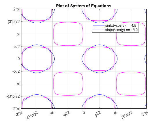
The solutions lie at the intersection of the two plots. This shows the system has repeated, periodic solutions. To solve this system of equations for the full solution set, use solve and set the ReturnConditions option to true.

S = solve(eqn1,eqn2,'ReturnConditions',true)

S = struct with fields:
             x: [2x1 sym]
             y: [2x1 sym]
    parameters: [z    z1]
    conditions: [2x1 sym]

solve returns a structure S with the fields S.x for the solution to x, S.y for the solution to y, S.parameters for the parameters in the solution, and S.conditions for the conditions on the solution. Elements of the same index in S.x, S.y, and S.conditions form a solution. Thus, S.x(1), S.y(1), and S.conditions(1) form one solution to the system of equations. The parameters in S.parameters can appear in all solutions.

Index into S to return the solutions, parameters, and conditions.

S.x

ans = 
$$\left(\begin{array}{c}{z}_1\\ z_1\end{array}\right)$$

S.y

ans = 
$$\left(\begin{array}{c}z\\ z\end{array}\right)$$

S.parameters

ans = $$\left(\begin{array}{cc}z& z_1\end{array}\right)$$

S.conditions

ans = 
$$\begin{array}{l}\left(\begin{array}{c}\left(\frac{z+\mathrm{acos}\left({\sigma }_3\right)}{2\hspace{0.17em}\pi }\in \mathbb{Z}\vee \frac{z-\mathrm{acos}\left({\sigma }_3\right)}{2\hspace{0.17em}\pi }\in \mathbb{Z}\right)\wedge \left(-\frac{\pi -z_1+{\sigma }_1}{2\hspace{0.17em}\pi }\in \mathbb{Z}\vee \frac{z_1+{\sigma }_1}{2\hspace{0.17em}\pi }\in \mathbb{Z}\right)\\ \left(\frac{z_1-\pi +\mathrm{asin}\left({\sigma }_3\right)}{2\hspace{0.17em}\pi }\in \mathbb{Z}\vee \frac{z_1-\mathrm{asin}\left({\sigma }_3\right)}{2\hspace{0.17em}\pi }\in \mathbb{Z}\right)\wedge \left(\frac{z+{\sigma }_2}{2\hspace{0.17em}\pi }\in \mathbb{Z}\vee \frac{z-{\sigma }_2}{2\hspace{0.17em}\pi }\in \mathbb{Z}\right)\end{array}\right)\\ \\ \mathrm{where}\\ \\ \mathrm{ }{\sigma }_1=\mathrm{asin}\left(\frac{\sqrt{6}}{10}-\frac{2}{5}\right)\\ \\ \mathrm{ }{\sigma }_2=\mathrm{acos}\left(\frac{2}{5}-\frac{\sqrt{6}}{10}\right)\\ \\ \mathrm{ }{\sigma }_3=\frac{\sqrt{6}}{10}+\frac{2}{5}\end{array}$$

Solve a System of Equations Under Conditions

To solve the system of equations under conditions, specify the conditions in the input to solve.

Solve the system of equations considered above for x and y in the interval -2*pi to 2*pi. Overlay the solutions on the plot using scatter.

Srange = solve(eqn1, eqn2, -2*pi < x, x < 2*pi, -2*pi < y, y < 2*pi, 'ReturnConditions', true);
scatter(Srange.x,Srange.y,'k')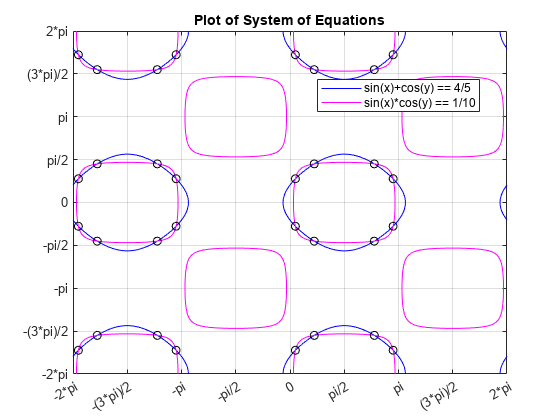

Work with Solutions, Parameters, and Conditions Returned by solve

You can use the solutions, parameters, and conditions returned by solve to find solutions within an interval or under additional conditions. This section has the same goal as the previous section, to solve the system of equations within a search range, but with a different approach. Instead of placing conditions directly, it shows how to work with the parameters and conditions returned by solve.

For the full solution S of the system of equations, find values of x and y in the interval -2*pi to 2*pi by solving the solutions S.x and S.y for the parameters S.parameters within that interval under the condition S.conditions.

Before solving for x and y in the interval, assume the conditions in S.conditions using assume so that the solutions returned satisfy the condition. Assume the conditions for the first solution.

assume(S.conditions(1))

Find the parameters in S.x and S.y.

paramx = intersect(symvar(S.x),S.parameters)

paramx = $$z_1$$

paramy = intersect(symvar(S.y),S.parameters)

paramy = $$z$$

Solve the first solution of x for the parameter paramx.

solparamx(1,:) = solve(S.x(1) > -2*pi, S.x(1) < 2*pi, paramx)

solparamx = 
$$\left(\begin{array}{cccc}\pi +\mathrm{asin}\left(\frac{\sqrt{6}}{10}-\frac{2}{5}\right)& \mathrm{asin}\left(\frac{\sqrt{6}}{10}-\frac{2}{5}\right)-\pi & -\mathrm{asin}\left(\frac{\sqrt{6}}{10}-\frac{2}{5}\right)& -2\hspace{0.17em}\pi -\mathrm{asin}\left(\frac{\sqrt{6}}{10}-\frac{2}{5}\right)\end{array}\right)$$

Similarly, solve the first solution of y for paramy.

solparamy(1,:) = solve(S.y(1) > -2*pi, S.y(1) < 2*pi, paramy)

solparamy = 
$$\left(\begin{array}{cccc}\mathrm{acos}\left(\frac{\sqrt{6}}{10}+\frac{2}{5}\right)& \mathrm{acos}\left(\frac{\sqrt{6}}{10}+\frac{2}{5}\right)-2\hspace{0.17em}\pi & -\mathrm{acos}\left(\frac{\sqrt{6}}{10}+\frac{2}{5}\right)& 2\hspace{0.17em}\pi -\mathrm{acos}\left(\frac{\sqrt{6}}{10}+\frac{2}{5}\right)\end{array}\right)$$

Clear the assumptions set by S.conditions(1) using assume. Call asumptions to check that the assumptions are cleared.

assume(S.parameters,'clear')
assumptions

 
ans =
 
Empty sym: 1-by-0
 

Assume the conditions for the second solution.

assume(S.conditions(2))

Solve the second solution to x and y for the parameters paramx and paramy.

solparamx(2,:) = solve(S.x(2) > -2*pi, S.x(2) < 2*pi, paramx)

solparamx = 
$$\begin{array}{l}\left(\begin{array}{cccc}\pi +{\sigma }_1& {\sigma }_1-\pi & -{\sigma }_1& -2\hspace{0.17em}\pi -{\sigma }_1\\ {\sigma }_2& \pi -{\sigma }_2& {\sigma }_2-2\hspace{0.17em}\pi & -\pi -{\sigma }_2\end{array}\right)\\ \\ \mathrm{where}\\ \\ \mathrm{ }{\sigma }_1=\mathrm{asin}\left(\frac{\sqrt{6}}{10}-\frac{2}{5}\right)\\ \\ \mathrm{ }{\sigma }_2=\mathrm{asin}\left(\frac{\sqrt{6}}{10}+\frac{2}{5}\right)\end{array}$$

solparamy(2,:) = solve(S.y(2) > -2*pi, S.y(2) < 2*pi, paramy)

solparamy = 
$$\begin{array}{l}\left(\begin{array}{cccc}{\sigma }_2& {\sigma }_2-2\hspace{0.17em}\pi & -{\sigma }_2& 2\hspace{0.17em}\pi -{\sigma }_2\\ {\sigma }_1& {\sigma }_1-2\hspace{0.17em}\pi & -{\sigma }_1& 2\hspace{0.17em}\pi -{\sigma }_1\end{array}\right)\\ \\ \mathrm{where}\\ \\ \mathrm{ }{\sigma }_1=\mathrm{acos}\left(\frac{2}{5}-\frac{\sqrt{6}}{10}\right)\\ \\ \mathrm{ }{\sigma }_2=\mathrm{acos}\left(\frac{\sqrt{6}}{10}+\frac{2}{5}\right)\end{array}$$

The first rows of paramx and paramy form the first solution to the system of equations, and the second rows form the second solution.

To find the values of x and y for these values of paramx and paramy, use subs to substitute for paramx and paramy in S.x and S.y.

solx(1,:) = subs(S.x(1), paramx, solparamx(1,:));
solx(2,:) = subs(S.x(2), paramx, solparamx(2,:))

solx = 
$$\begin{array}{l}\left(\begin{array}{cccc}\pi +{\sigma }_1& {\sigma }_1-\pi & -{\sigma }_1& -2\hspace{0.17em}\pi -{\sigma }_1\\ {\sigma }_2& \pi -{\sigma }_2& {\sigma }_2-2\hspace{0.17em}\pi & -\pi -{\sigma }_2\end{array}\right)\\ \\ \mathrm{where}\\ \\ \mathrm{ }{\sigma }_1=\mathrm{asin}\left(\frac{\sqrt{6}}{10}-\frac{2}{5}\right)\\ \\ \mathrm{ }{\sigma }_2=\mathrm{asin}\left(\frac{\sqrt{6}}{10}+\frac{2}{5}\right)\end{array}$$

soly(1,:) = subs(S.y(1), paramy, solparamy(1,:));
soly(2,:) = subs(S.y(2), paramy, solparamy(2,:))

soly = 
$$\begin{array}{l}\left(\begin{array}{cccc}{\sigma }_2& {\sigma }_2-2\hspace{0.17em}\pi & -{\sigma }_2& 2\hspace{0.17em}\pi -{\sigma }_2\\ {\sigma }_1& {\sigma }_1-2\hspace{0.17em}\pi & -{\sigma }_1& 2\hspace{0.17em}\pi -{\sigma }_1\end{array}\right)\\ \\ \mathrm{where}\\ \\ \mathrm{ }{\sigma }_1=\mathrm{acos}\left(\frac{2}{5}-\frac{\sqrt{6}}{10}\right)\\ \\ \mathrm{ }{\sigma }_2=\mathrm{acos}\left(\frac{\sqrt{6}}{10}+\frac{2}{5}\right)\end{array}$$

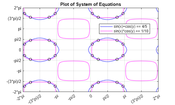
Note that solx and soly are the two sets of solutions to x and to y. The full sets of solutions to the system of equations are the two sets of points formed by all possible combinations of the values in solx and soly.

Plot these two sets of points using scatter. Overlay them on the plot of the equations. As expected, the solutions appear at the intersection of the plots of the two equations.

for i = 1:length(solx(1,:))
    for j = 1:length(soly(1,:))
        scatter(solx(1,i), soly(1,j), 'k')
        scatter(solx(2,i), soly(2,j), 'k')
    end
end

Convert Symbolic Results to Numeric Values

Symbolic calculations provide exact accuracy, while numeric calculations are approximations. Despite this loss of accuracy, you might need to convert symbolic results to numeric approximations for use in numeric calculations. For a high-accuracy conversion, use variable-precision arithmetic provided by the vpa function. For standard accuracy and better performance, convert to double precision using double.

Use vpa to convert the symbolic solutions solx and soly to numeric form.

vpa(solx)

ans = 
$$\left(\begin{array}{cccc}2.9859135500977407388300518406219& -3.2972717570818457380952349259371& 0.15567910349205249963259154265761& -6.1275062036875339772926952239014\\ 0.70095651347102524787213653614929& 2.4406361401187679905905068471302& -5.5822287937085612290531502304097& -3.8425491670608184863347799194288\end{array}\right)$$

vpa(soly)

ans = 
$$\left(\begin{array}{cccc}0.86983981332387137135918515549046& -5.4133454938557151055661016110685& -0.86983981332387137135918515549046& 5.4133454938557151055661016110685\\ 1.4151172233028441195987301489821& -4.8680680838767423573265566175769& -1.4151172233028441195987301489821& 4.8680680838767423573265566175769\end{array}\right)$$

Simplify Complicated Results and Improve Performance

If results look complicated, solve is stuck, or if you want to improve performance, see, Troubleshoot Equation Solutions from solve Function.

×

Beispiel öffnen

Sie haben eine geänderte Version dieses Beispiels. Möchten Sie dieses Beispiel mit Ihren Änderungen öffnen?

Nein, geänderte Version überschreiben Ja