cvpredict
Description
predictedY = cvpredict(CVMdl)CVMdl. For each partition window in
CVMdl.Partition and each horizon step in
CVMdl.Horizon, the function predicts the response for test observations
by using a model trained on training observations. If an observation is in more than one
test set, the function returns the prediction for that observation, averaged over all test
sets.
Examples
Create a cross-validated direct forecasting model using expanding window cross-validation. To evaluate the performance of the model:
Compute the mean squared error (MSE) on each test set using the
cvlossobject function.For each test set, compare the true response values to the predicted response values using the
cvpredictobject function.
Load the sample file TemperatureData.csv, which contains average daily temperature from January 2015 through July 2016. Read the file into a table. Observe the first eight observations in the table.
Tbl = readtable("TemperatureData.csv");
head(Tbl)
Year Month Day TemperatureF
____ ___________ ___ ____________
2015 {'January'} 1 23
2015 {'January'} 2 31
2015 {'January'} 3 25
2015 {'January'} 4 39
2015 {'January'} 5 29
2015 {'January'} 6 12
2015 {'January'} 7 10
2015 {'January'} 8 4
Create a datetime variable t that contains the year, month, and day information for each observation in Tbl.
numericMonth = month(datetime(Tbl.Month, ...
    InputFormat="MMMM",Locale="en_US"));
t = datetime(Tbl.Year,numericMonth,Tbl.Day);
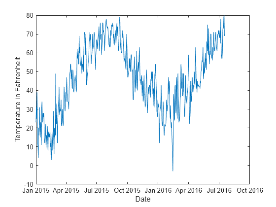
Plot the temperature values in Tbl over time.
plot(t,Tbl.TemperatureF)
xlabel("Date")
ylabel("Temperature in Fahrenheit")
Create a direct forecasting model by using the data in Tbl. Train the model using a bagged ensemble of trees. All three of the predictors (Year, Month, and Day) are leading predictors because their future values are known. To create new predictors by shifting the leading predictor and response variables backward in time, specify the leading predictor lags and the response variable lags.
Mdl = directforecaster(Tbl,"TemperatureF", ...
    Learner="bag", ...
    LeadingPredictors="all",LeadingPredictorLags={0:1,0:1,0:7}, ...
    ResponseLags=1:7)
Mdl =
  DirectForecaster

                  Horizon: 1
             ResponseLags: [1 2 3 4 5 6 7]
        LeadingPredictors: [1 2 3]
     LeadingPredictorLags: {[0 1]  [0 1]  [0 1 2 3 4 5 6 7]}
             ResponseName: 'TemperatureF'
           PredictorNames: {'Year'  'Month'  'Day'}
    CategoricalPredictors: 2
                 Learners: {[1×1 classreg.learning.regr.CompactRegressionEnsemble]}
                   MaxLag: 7
          NumObservations: 565


  Properties, Methods
Mdl is a DirectForecaster model object. By default, the horizon is one step ahead. That is, Mdl predicts a value that is one step into the future.
Partition the time series data in Tbl using an expanding window cross-validation scheme. Create three training sets and three test sets, where each test set has 100 observations. Note that each observation in Tbl is in at most one test set.
CVPartition = tspartition(size(Mdl.X,1),"ExpandingWindow",3, ...
    TestSize=100)
CVPartition =
  tspartition

               Type: 'expanding-window'
    NumObservations: 565
        NumTestSets: 3
          TrainSize: [265 365 465]
           TestSize: [100 100 100]
           StepSize: 100


  Properties, Methods
The training sets increase in size from 265 observations in the first window to 465 observations in the third window.
Create a cross-validated direct forecasting model using the partition specified in CVPartition. Inspect the Learners property of the resulting CVMdl object.
CVMdl = crossval(Mdl,CVPartition)
CVMdl =
  PartitionedDirectForecaster

                Partition: [1×1 tspartition]
                  Horizon: 1
             ResponseLags: [1 2 3 4 5 6 7]
        LeadingPredictors: [1 2 3]
     LeadingPredictorLags: {[0 1]  [0 1]  [0 1 2 3 4 5 6 7]}
             ResponseName: 'TemperatureF'
           PredictorNames: {'Year'  'Month'  'Day'}
    CategoricalPredictors: 2
                 Learners: {3×1 cell}
                   MaxLag: 7
          NumObservations: 565


  Properties, Methods
CVMdl.Learners
ans=3×1 cell array
    {1×1 timeseries.forecaster.CompactDirectForecaster}
    {1×1 timeseries.forecaster.CompactDirectForecaster}
    {1×1 timeseries.forecaster.CompactDirectForecaster}
CVMdl is a PartitionedDirectForecaster model object. The crossval function trains CVMdl.Learners{1} using the observations in the first training set, CVMdl.Learner{2} using the observations in the second training set, and CVMdl.Learner{3} using the observations in the third training set.
Compute the average test set MSE.
averageMSE = cvloss(CVMdl)
averageMSE =
53.3480
To obtain more information, compute the MSE for each test set.
individualMSE = cvloss(CVMdl,Mode="individual")individualMSE = 3×1
44.1352
84.0695
31.8393
The models trained on the first and third training sets seem to perform better than the model trained on the second training set.
For each test set observation, predict the temperature value using the corresponding model in CVMdl.Learners.
predictedY = cvpredict(CVMdl);
predictedY(260:end,:)
ans=306×1 table
    TemperatureF_Step1
    __________________

             NaN
             NaN
             NaN
             NaN
             NaN
             NaN
          50.963
          57.363
           57.04
          60.705
          59.606
          58.302
          58.023
           61.39
          67.229
          61.083
      ⋮
Only the last 300 observations appear in any test set. For observations that do not appear in a test set, the predicted response value is NaN.
For each test set, plot the true response values and the predicted response values.
tiledlayout(3,1)

nexttile
idx1 = test(CVPartition,1);
plot(t(idx1),Tbl.TemperatureF(idx1))
hold on
plot(t(idx1),predictedY.TemperatureF_Step1(idx1))
legend("True Response","Predicted Response", ...
    Location="eastoutside")
xlabel("Date")
ylabel("Temperature")
title("Test Set 1")
hold off

nexttile
idx2 = test(CVPartition,2);
plot(t(idx2),Tbl.TemperatureF(idx2))
hold on
plot(t(idx2),predictedY.TemperatureF_Step1(idx2))
legend("True Response","Predicted Response", ...
    Location="eastoutside")
xlabel("Date")
ylabel("Temperature")
title("Test Set 2")
hold off

nexttile
idx3 = test(CVPartition,3);
plot(t(idx3),Tbl.TemperatureF(idx3))
hold on
plot(t(idx3),predictedY.TemperatureF_Step1(idx3))
legend("True Response","Predicted Response", ...
    Location="eastoutside")
xlabel("Date")
ylabel("Temperature")
title("Test Set 3")
hold off
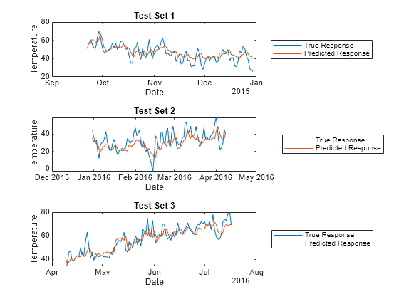
Overall, the cross-validated direct forecasting model is able to predict the trend in temperatures. If you are satisfied with the performance of the cross-validated model, you can use the full DirectForecaster model Mdl for forecasting at time steps beyond the available data.
Create a partitioned direct forecasting model using holdout validation. To evaluate the performance of the model:
At each horizon step, compute the root relative squared error (RRSE) on the test set using the
cvlossobject function.At each horizon step, compare the true response values to the predicted response values using the
cvpredictobject function.
Load the sample file TemperatureData.csv, which contains average daily temperature from January 2015 through July 2016. Read the file into a table. Observe the first eight observations in the table.
Tbl = readtable("TemperatureData.csv");
head(Tbl)
Year Month Day TemperatureF
____ ___________ ___ ____________
2015 {'January'} 1 23
2015 {'January'} 2 31
2015 {'January'} 3 25
2015 {'January'} 4 39
2015 {'January'} 5 29
2015 {'January'} 6 12
2015 {'January'} 7 10
2015 {'January'} 8 4
Create a datetime variable t that contains the year, month, and day information for each observation in Tbl.
numericMonth = month(datetime(Tbl.Month, ...
    InputFormat="MMMM",Locale="en_US"));
t = datetime(Tbl.Year,numericMonth,Tbl.Day);
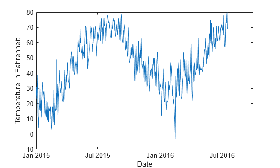
Plot the temperature values in Tbl over time.
plot(t,Tbl.TemperatureF)
xlabel("Date")
ylabel("Temperature in Fahrenheit")
Create a direct forecasting model by using the data in Tbl. Specify the horizon steps as one, two, and three steps ahead. Train a model at each horizon using a bagged ensemble of trees. All three of the predictors (Year, Month, and Day) are leading predictors because their future values are known. To create new predictors by shifting the leading predictor and response variables backward in time, specify the leading predictor lags and the response variable lags.
rng("default")
Mdl = directforecaster(Tbl,"TemperatureF", ...
    Horizon=1:3,Learner="bag", ...
    LeadingPredictors="all",LeadingPredictorLags={0:1,0:1,0:7}, ...
    ResponseLags=1:7)
Mdl =
  DirectForecaster

                  Horizon: [1 2 3]
             ResponseLags: [1 2 3 4 5 6 7]
        LeadingPredictors: [1 2 3]
     LeadingPredictorLags: {[0 1]  [0 1]  [0 1 2 3 4 5 6 7]}
             ResponseName: 'TemperatureF'
           PredictorNames: {'Year'  'Month'  'Day'}
    CategoricalPredictors: 2
                 Learners: {3×1 cell}
                   MaxLag: 7
          NumObservations: 565


  Properties, Methods
Mdl is a DirectForecaster model object. Mdl consists of three regression models: Mdl.Learners{1}, which predicts one step ahead; Mdl.Learners{2}, which predicts two steps ahead; and Mdl.Learners{3}, which predicts three steps ahead.
Partition the time series data in Tbl using a holdout validation scheme. Reserve 20% of the observations for testing.
holdoutPartition = tspartition(size(Mdl.X,1),"Holdout",0.20)holdoutPartition =
tspartition
Type: 'holdout'
NumObservations: 565
NumTestSets: 1
TrainSize: 452
TestSize: 113
Properties, Methods
The test set consists of the latest 113 observations.
Create a partitioned direct forecasting model using the partition specified in holdoutPartition.
holdoutMdl = crossval(Mdl,holdoutPartition)
holdoutMdl =
  PartitionedDirectForecaster

                Partition: [1×1 tspartition]
                  Horizon: [1 2 3]
             ResponseLags: [1 2 3 4 5 6 7]
        LeadingPredictors: [1 2 3]
     LeadingPredictorLags: {[0 1]  [0 1]  [0 1 2 3 4 5 6 7]}
             ResponseName: 'TemperatureF'
           PredictorNames: {'Year'  'Month'  'Day'}
    CategoricalPredictors: 2
                 Learners: {[1×1 timeseries.forecaster.CompactDirectForecaster]}
                   MaxLag: 7
          NumObservations: 565


  Properties, Methods
holdoutMdl is a PartitionedDirectForecaster model object. Because holdoutMdl uses holdout validation rather than a cross-validation scheme, the Learners property of the object contains one CompactDirectForecaster model only.
Like Mdl, holdoutMdl contains three regression models. The crossval function trains holdoutMdl.Learners{1}.Learners{1}, holdoutMdl.Learners{1}.Learners{2}, and holdoutMdl.Learners{1}.Learners{3} using the same training data. However, the three models use different response variables because each model predicts values for a different horizon step.
holdoutMdl.Learners{1}.Learners{1}.ResponseNameans = 'TemperatureF_Step1'
holdoutMdl.Learners{1}.Learners{2}.ResponseNameans = 'TemperatureF_Step2'
holdoutMdl.Learners{1}.Learners{3}.ResponseNameans = 'TemperatureF_Step3'
Compute the root relative squared error (RRSE) on the test data at each horizon step. Use the helper function computeRRSE (shown at the end of this example). The RRSE indicates how well a model performs relative to the simple model, which always predicts the average of the true values. In particular, when the RRSE is less than 1, the model performs better than the simple model.
holdoutRRSE = cvloss(holdoutMdl,LossFun=@computeRRSE)
holdoutRRSE = 1×3

    0.4797    0.5889    0.6103
At each horizon, the direct forecasting model seems to perform better than the simple model.
For each test set observation, predict the temperature value using the corresponding model in holdoutMdl.Learners.
predictedY = cvpredict(holdoutMdl);
predictedY(450:end,:)
ans=116×3 table
    TemperatureF_Step1    TemperatureF_Step2    TemperatureF_Step3
    __________________    __________________    __________________

             NaN                   NaN                   NaN
             NaN                   NaN                   NaN
             NaN                   NaN                   NaN
          41.063                39.758                41.234
          33.721                36.507                37.719
          36.987                35.133                37.719
          38.644                34.598                36.444
          38.917                34.576                36.275
          45.888                37.005                 38.34
          48.516                42.762                 41.05
          44.882                46.816                43.881
          35.057                45.301                47.048
            31.1                41.473                42.948
          31.817                37.314                42.946
          33.166                38.419                  41.3
          40.279                38.432                40.533
      ⋮
Recall that only the latest 113 observations appear in the test set. For observations that do not appear in the test set, the predicted response value is NaN.
For each test set, plot the true response values and the predicted response values.
tiledlayout(3,1)

idx = test(holdoutPartition);

nexttile
plot(t(idx),Tbl.TemperatureF(idx))
hold on
plot(t(idx),predictedY.TemperatureF_Step1(idx))
legend("True Response","Predicted Response", ...
    Location="eastoutside")
xlabel("Date")
ylabel("Temperature")
title("Horizon 1")
hold off

nexttile
plot(t(idx),Tbl.TemperatureF(idx))
hold on
plot(t(idx),predictedY.TemperatureF_Step2(idx))
legend("True Response","Predicted Response", ...
    Location="eastoutside")
xlabel("Date")
ylabel("Temperature")
title("Horizon 2")
hold off

nexttile
plot(t(idx),Tbl.TemperatureF(idx))
hold on
plot(t(idx),predictedY.TemperatureF_Step3(idx))
legend("True Response","Predicted Response", ...
    Location="eastoutside")
xlabel("Date")
ylabel("Temperature")
title("Horizon 3")
hold off
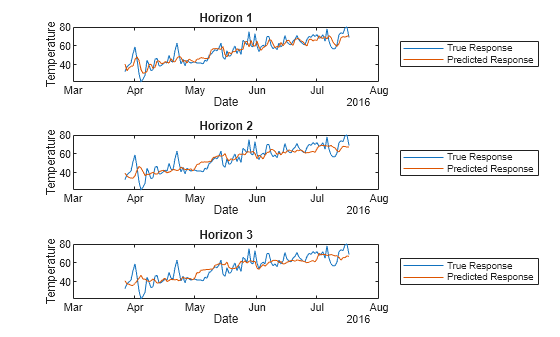
Overall, holdoutMdl is able to predict the trend in temperatures, although it seems to perform best when forecasting one step ahead. If you are satisfied with the performance of the partitioned model, you can use the full DirectForecaster model Mdl for forecasting at time steps beyond the available data.
Helper Function
The helper function computeRRSE computes the RRSE given the true response variable trueY and the predicted values predY. This code creates the computeRRSE helper function.
function rrse = computeRRSE(trueY,predY)
    error = trueY(:) - predY(:);
    meanY = mean(trueY(:),"omitnan");
    rrse = sqrt(sum(error.^2,"omitnan")/sum((trueY(:) - meanY).^2,"omitnan"));
end
Input Arguments
Output Arguments
Version History
Introduced in R2023b