Linear Regression with Categorical Covariates

This example shows how to perform a regression with categorical covariates using categorical arrays and fitlm.

Load sample data.

load carsmall

The variable MPG contains measurements on the miles per gallon of 100 sample cars. The model year of each car is in the variable Model_Year, and Weight contains the weight of each car.

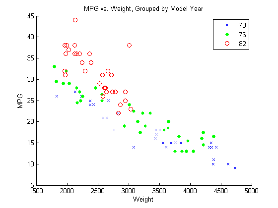
Plot grouped data.

Draw a scatter plot of MPG against Weight, grouped by model year.

figure()
gscatter(Weight,MPG,Model_Year,'bgr','x.o')
title('MPG vs. Weight, Grouped by Model Year')

Scatter plot of MPG versus Weight. The observations are grouped by model year. Observations corresponding to 1970, 1976, and 1982 are plotted as blue X markers, green points, and red O markers, respectively.

The grouping variable, Model_Year, has three unique values, 70, 76, and 82, corresponding to model years 1970, 1976, and 1982.

Create table and categorical array.

Create a table that contains the variables MPG, Weight, and Model_Year. Convert the variable Model_Year to a categorical array.

cars = table(MPG,Weight,Model_Year);
cars.Model_Year = categorical(cars.Model_Year);

Fit a regression model.

Fit a regression model using fitlm with MPG as the dependent variable, and Weight and Model_Year as the independent variables. Because Model_Year is a categorical covariate with three levels, it should enter the model as two indicator variables.

The scatter plot suggests that the slope of MPG against Weight might differ for each model year. To assess this, include weight-year interaction terms.

The proposed model is

$E (M P G) = β_{0} + β_{1} W e i g h t + β_{2} I [1976] + β_{3} I [1982] + β_{4} W e i g h t \times I [1976] + β_{5} W e i g h t \times I [1982],$

where I[1976] and I[1982] are dummy variables indicating the model years 1976 and 1982, respectively. I[1976] takes the value 1 if model year is 1976 and takes the value 0 if it is not. I[1982] takes the value 1 if model year is 1982 and takes the value 0 if it is not. In this model, 1970 is the reference year.

fit = fitlm(cars,'MPG~Weight*Model_Year')

fit = 


Linear regression model:
    MPG ~ 1 + Weight*Model_Year

Estimated Coefficients:
                             Estimate          SE    
                            ___________    __________

    (Intercept)                  37.399        2.1466
    Weight                   -0.0058437    0.00061765
    Model_Year_76                4.6903        2.8538
    Model_Year_82                21.051         4.157
    Weight:Model_Year_76    -0.00082009    0.00085468
    Weight:Model_Year_82     -0.0050551     0.0015636


                             tStat        pValue  
                            ________    __________

    (Intercept)               17.423    2.8607e-30
    Weight                   -9.4612    4.6077e-15
    Model_Year_76             1.6435       0.10384
    Model_Year_82             5.0641    2.2364e-06
    Weight:Model_Year_76    -0.95953       0.33992
    Weight:Model_Year_82     -3.2329     0.0017256


Number of observations: 94, Error degrees of freedom: 88
Root Mean Squared Error: 2.79
R-squared: 0.886,  Adjusted R-Squared: 0.88
F-statistic vs. constant model: 137, p-value = 5.79e-40

The regression output shows:

fitlm recognizes Model_Year as a categorical variable, and constructs the required indicator (dummy) variables. By default, the first level, 70, is the reference group (use reordercats to change the reference group).
The model specification, MPG~Weight*Model_Year, specifies the first-order terms for Weight and Model_Year, and all interactions.
The model R² = 0.886, meaning the variation in miles per gallon is reduced by 88.6% when you consider weight, model year, and their interactions.

The fitted model is

$M \hat{P} G = 37.4 - 0.006 W e i g h t + 4.7 I [1976] + 21.1 I [1982] - 0.0008 W e i g h t \times I [1976] - 0.005 W e i g h t \times I [1982] .$

Thus, the estimated regression equations for the model years are as follows.

Model Year	Predicted MPG Against Weight
1970	$M \hat{P} G = 37.4 - 0.006 W e i g h t$
1976	$M \hat{P} G = (37.4 + 4.7) - (0.006 + 0.0008) W e i g h t$
1982	$M \hat{P} G = (37.4 + 21.1) - (0.006 + 0.005) W e i g h t$

Model Year

Predicted MPG Against Weight

1970

$M \hat{P} G = 37.4 - 0.006 W e i g h t$

1976

$M \hat{P} G = (37.4 + 4.7) - (0.006 + 0.0008) W e i g h t$

1982

$M \hat{P} G = (37.4 + 21.1) - (0.006 + 0.005) W e i g h t$

The relationship between MPG and Weight has an increasingly negative slope as the model year increases.

Plot fitted regression lines.

Plot the data and fitted regression lines.

w = linspace(min(Weight),max(Weight));

figure()
gscatter(Weight,MPG,Model_Year,'bgr','x.o')
line(w,feval(fit,w,'70'),'Color','b','LineWidth',2)
line(w,feval(fit,w,'76'),'Color','g','LineWidth',2)
line(w,feval(fit,w,'82'),'Color','r','LineWidth',2)
title('Fitted Regression Lines by Model Year')

Test for different slopes.

Test for significant differences between the slopes. This is equivalent to testing the hypothesis

$\begin{array}{l} H_{0} : β_{4} = β_{5} = 0 \\ H_{A} : β_{i} \neq 0 for at least one i . \end{array}$

anova(fit)

ans = 

                         SumSq     DF    MeanSq    F         pValue    
    Weight               2050.2     1    2050.2    263.87    3.2055e-28
    Model_Year           807.69     2    403.84    51.976    1.2494e-15
    Weight:Model_Year    81.219     2    40.609    5.2266     0.0071637
    Error                683.74    88    7.7698

This output shows that the p-value for the test is 0.0072 (from the interaction row, Weight:Model_Year), so the null hypothesis is rejected at the 0.05 significance level. The value of the test statistic is 5.2266. The numerator degrees of freedom for the test is 2, which is the number of coefficients in the null hypothesis.

There is sufficient evidence that the slopes are not equal for all three model years.