Create and Visualize Discriminant Analysis Classifier
This example shows how to perform linear and quadratic classification of Fisher iris data.
Load the sample data.
load fisheririsThe column vector, species, consists of iris flowers of three different species, setosa, versicolor, virginica. The double matrix meas consists of four types of measurements on the flowers, the length and width of sepals and petals in centimeters, respectively.
Use petal length (third column in meas) and petal width (fourth column in meas) measurements. Save these as variables PL and PW, respectively.
PL = meas(:,3);
PW = meas(:,4);
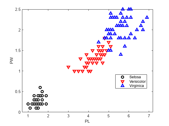
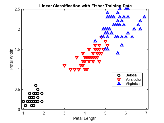
Plot the data, showing the classification, that is, create a scatter plot of the measurements, grouped by species.
h1 = gscatter(PL,PW,species,'krb','ov^',[],'off');
h1(1).LineWidth = 2;
h1(2).LineWidth = 2;
h1(3).LineWidth = 2;
legend('Setosa','Versicolor','Virginica','Location','best')
hold on
Create a linear classifier.
X = [PL,PW];
MdlLinear = fitcdiscr(X,species);
Retrieve the coefficients for the linear boundary between the second and third classes.
MdlLinear.ClassNames([2 3])
ans = 2×1 cell
    {'versicolor'}
    {'virginica' }
K = MdlLinear.Coeffs(2,3).Const;
L = MdlLinear.Coeffs(2,3).Linear;
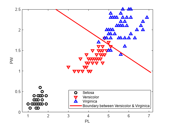
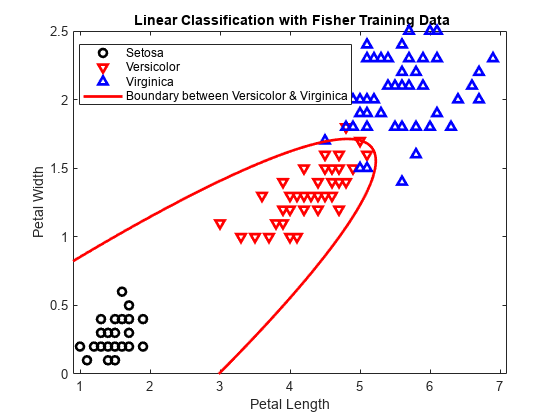
Plot the curve that separates the second and third classes.
f = @(x1,x2) K + L(1)*x1 + L(2)*x2;
h2 = fimplicit(f,[.9 7.1 0 2.5]);
h2.Color = 'r';
h2.LineWidth = 2;
h2.DisplayName = 'Boundary between Versicolor & Virginica';
Retrieve the coefficients for the linear boundary between the first and second classes.
MdlLinear.ClassNames([1 2])
ans = 2×1 cell
    {'setosa'    }
    {'versicolor'}
K = MdlLinear.Coeffs(1,2).Const;
L = MdlLinear.Coeffs(1,2).Linear;
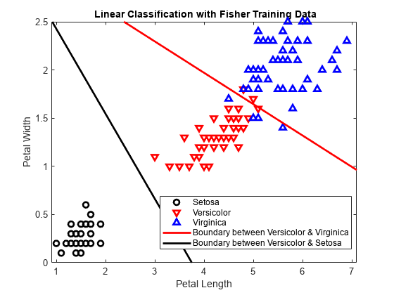
Plot the curve that separates the first and second classes.
f = @(x1,x2) K + L(1)*x1 + L(2)*x2;
h3 = fimplicit(f,[.9 7.1 0 2.5]);
h3.Color = 'k';
h3.LineWidth = 2;
h3.DisplayName = 'Boundary between Versicolor & Setosa';
axis([.9 7.1 0 2.5])
xlabel('Petal Length')
ylabel('Petal Width')
title('{\bf Linear Classification with Fisher Training Data}')
Create a quadratic discriminant classifier.
MdlQuadratic = fitcdiscr(X,species,'DiscrimType','quadratic');
Remove the linear boundaries from the plot.
delete(h2);
delete(h3);
Retrieve the coefficients for the quadratic boundary between the second and third classes.
MdlQuadratic.ClassNames([2 3])
ans = 2×1 cell
    {'versicolor'}
    {'virginica' }
K = MdlQuadratic.Coeffs(2,3).Const;
L = MdlQuadratic.Coeffs(2,3).Linear;
Q = MdlQuadratic.Coeffs(2,3).Quadratic;
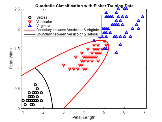
Plot the curve that separates the second and third classes.
f = @(x1,x2) K + L(1)*x1 + L(2)*x2 + Q(1,1)*x1.^2 + ...
    (Q(1,2)+Q(2,1))*x1.*x2 + Q(2,2)*x2.^2;
h2 = fimplicit(f,[.9 7.1 0 2.5]);
h2.Color = 'r';
h2.LineWidth = 2;
h2.DisplayName = 'Boundary between Versicolor & Virginica';
Retrieve the coefficients for the quadratic boundary between the first and second classes.
MdlQuadratic.ClassNames([1 2])
ans = 2×1 cell
    {'setosa'    }
    {'versicolor'}
K = MdlQuadratic.Coeffs(1,2).Const;
L = MdlQuadratic.Coeffs(1,2).Linear;
Q = MdlQuadratic.Coeffs(1,2).Quadratic;
Plot the curve that separates the first and second and classes.
f = @(x1,x2) K + L(1)*x1 + L(2)*x2 + Q(1,1)*x1.^2 + ...
    (Q(1,2)+Q(2,1))*x1.*x2 + Q(2,2)*x2.^2;
h3 = fimplicit(f,[.9 7.1 0 1.02]); % Plot the relevant portion of the curve.
h3.Color = 'k';
h3.LineWidth = 2;
h3.DisplayName = 'Boundary between Versicolor & Setosa';
axis([.9 7.1 0 2.5])
xlabel('Petal Length')
ylabel('Petal Width')
title('{\bf Quadratic Classification with Fisher Training Data}')
hold off