Main Content

incrementalLearner

Convert linear model for binary classification to incremental learner

Since R2020b

Description

example

IncrementalMdl = incrementalLearner(Mdl) returns a binary classification linear model for incremental learning, IncrementalMdl, using the traditionally trained linear model object or linear model template object in Mdl.

If you specify a traditionally trained model, then its property values reflect the knowledge gained from Mdl (parameters and hyperparameters of the model). Therefore, IncrementalMdl can predict labels given new observations, and it is warm, meaning that its predictive performance is tracked.

example

IncrementalMdl = incrementalLearner(Mdl,Name,Value) uses additional options specified by one or more name-value arguments. Some options require you to train IncrementalMdl before its predictive performance is tracked. For example, 'MetricsWarmupPeriod',50,'MetricsWindowSize',100 specifies a preliminary incremental training period of 50 observations before performance metrics are tracked, and specifies processing 100 observations before updating the window performance metrics.

Examples

collapse all

Train a linear classification model for binary learning by using fitclinear, and then convert it to an incremental learner.

Load and Preprocess Data

Load the human activity data set.

load humanactivity

For details on the data set, enter Description at the command line.

Responses can be one of five classes: Sitting, Standing, Walking, Running, or Dancing. Dichotomize the response by identifying whether the subject is moving (actid > 2).

Y = actid > 2;

Train Linear Classification Model

Fit a linear classification model to the entire data set.

TTMdl = fitclinear(feat,Y)
TTMdl = 
  ClassificationLinear
      ResponseName: 'Y'
        ClassNames: [0 1]
    ScoreTransform: 'none'
              Beta: [60x1 double]
              Bias: -0.2005
            Lambda: 4.1537e-05
           Learner: 'svm'


TTMdl is a ClassificationLinear model object representing a traditionally trained linear classification model.

Convert Trained Model

Convert the traditionally trained linear classification model to a binary classification linear model for incremental learning.

IncrementalMdl = incrementalLearner(TTMdl)
IncrementalMdl = 
  incrementalClassificationLinear

            IsWarm: 1
           Metrics: [1x2 table]
        ClassNames: [0 1]
    ScoreTransform: 'none'
              Beta: [60x1 double]
              Bias: -0.2005
           Learner: 'svm'


IncrementalMdl is an incrementalClassificationLinear model object prepared for incremental learning using SVM.

  • The incrementalLearner function initializes the incremental learner by passing learned coefficients to it, along with other information TTMdl extracted from the training data.

  • IncrementalMdl is warm (IsWarm is 1), which means that incremental learning functions can start tracking performance metrics.

  • incrementalClassificationLinear trains the model using the adaptive scale-invariant solver, whereas fitclinear trained TTMdl using the BFGS solver.

Predict Responses

An incremental learner created from converting a traditionally trained model can generate predictions without further processing.

Predict classification scores for all observations using both models.

[~,ttscores] = predict(TTMdl,feat);
[~,ilscores] = predict(IncrementalMdl,feat);
compareScores = norm(ttscores(:,1) - ilscores(:,1))
compareScores = 0

The difference between the scores generated by the models is 0.

If you train a linear classification model using the SGD or ASGD solver, incrementalLearner preserves the solver, linear model type, and associated hyperparameter values when it converts the linear classification model.

Load the human activity data set.

load humanactivity

For details on the data set, enter Description at the command line.

Responses can be one of five classes: Sitting, Standing, Walking, Running, or Dancing. Dichotomize the response by identifying whether the subject is moving (actid > 2).

Y = actid > 2;

Randomly split the data in half: the first half for training a model traditionally, and the second half for incremental learning.

n = numel(Y);
rng(1) % For reproducibility
cvp = cvpartition(n,'Holdout',0.5);
idxtt = training(cvp);
idxil = test(cvp);

% First half of data 
Xtt = feat(idxtt,:);
Ytt = Y(idxtt);

% Second half of data
Xil = feat(idxil,:);
Yil = Y(idxil);

Create a set of 11 logarithmically spaced regularization strengths from 10-6 through 10-0.5.

Lambda = logspace(-6,-0.5,11);

Because the variables are on different scales, use implicit expansion to standardize the predictor data.

Xtt = (Xtt - mean(Xtt))./std(Xtt);

Tune the L2 regularization parameter by applying 5-fold cross-validation. Specify the standard SGD solver.

TTCVMdl = fitclinear(Xtt,Ytt,'KFold',5,'Learner','logistic',...
    'Solver','sgd','Lambda',Lambda);

TTCVMdl is a ClassificationPartitionedLinear model representing the five models created during cross-validation (see TTCVMdl.Trained). The cross-validation procedure includes training with each specified regularization value.

Compute the cross-validated classification error for each model and regularization.

cvloss = kfoldLoss(TTCVMdl)
cvloss = 1×11

    0.0054    0.0039    0.0034    0.0033    0.0030    0.0027    0.0027    0.0031    0.0036    0.0056    0.0077

cvloss contains the test-sample classification loss for each regularization value in Lamba.

Select the regularization value that minimizes the classification error. Train the model again using the selected regularization value.

[~,idxmin] = min(cvloss);
TTMdl = fitclinear(Xtt,Ytt,'Learner','logistic','Solver','sgd',...
    'Lambda',Lambda(idxmin));

TTMdl is a ClassificationLinear model.

Convert the traditionally trained linear classification model to a binary classification linear model for incremental learning.

IncrementalMdl = incrementalLearner(TTMdl);

IncrementalMdl is an incrementalClassificationLinear model object. incrementalLearner passes the solver and regularization strength, among other information learned from training TTMdl, to IncrementalMdl.

Fit the incremental model to the second half of the data by using the fit function. At each iteration:

  • Simulate a data stream by processing 10 observations at a time.

  • Overwrite the previous incremental model with a new one fitted to the incoming observations.

  • Store β1 to see how it evolves during training.

% Preallocation
nil = numel(Yil);
numObsPerChunk = 10;
nchunk = floor(nil/numObsPerChunk);
learnrate = [IncrementalMdl.LearnRate; zeros(nchunk,1)];
beta1 = [IncrementalMdl.Beta(1); zeros(nchunk,1)];

% Incremental fitting
for j = 1:nchunk
    ibegin = min(nil,numObsPerChunk*(j-1) + 1);
    iend   = min(nil,numObsPerChunk*j);
    idx = ibegin:iend;
    IncrementalMdl = fit(IncrementalMdl,Xil(idx,:),Yil(idx));
    beta1(j + 1) = IncrementalMdl.Beta(1);
end

IncrementalMdl is an incrementalClassificationLinear model object trained on all the data in the stream.

Plot β1 to see how it evolved.

plot(beta1)
ylabel('\beta_1') 
xline(IncrementalMdl.EstimationPeriod/numObsPerChunk,'r-.')
xlabel('Iteration')

β1 
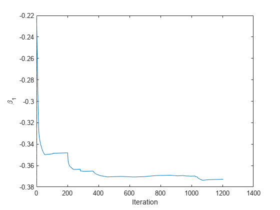
has an initial value of –0.22 and approaches a value of –0.37 during incremental fitting.

Use a trained linear classification model to initialize an incremental learner. Prepare the incremental learner by specifying a metrics warm-up period, during which the updateMetricsAndFit function only fits the model. Specify a metrics window size of 500 observations.

Load the human activity data set.

load humanactivity

For details on the data set, enter Description at the command line.

Responses can be one of five classes: Sitting, Standing, Walking, Running, and Dancing. Dichotomize the response by identifying whether the subject is moving (actid > 2).

Y = actid > 2;

Because the data set is grouped by activity, shuffle it for simplicity. Then, randomly split the data in half: the first half for training a model traditionally, and the second half for incremental learning.

n = numel(Y);

rng(1) % For reproducibility
cvp = cvpartition(n,'Holdout',0.5);
idxtt = training(cvp);
idxil = test(cvp);
shuffidx = randperm(n);
X = feat(shuffidx,:);
Y = Y(shuffidx);

% First half of data
Xtt = X(idxtt,:);
Ytt = Y(idxtt);

% Second half of data
Xil = X(idxil,:);
Yil = Y(idxil);

Fit a linear classification model to the first half of the data.

TTMdl = fitclinear(Xtt,Ytt);

Convert the traditionally trained linear classification model to a binary classification linear model for incremental learning. Specify the following:

  • A performance metrics warm-up period of 2000 observations

  • A metrics window size of 500 observations

  • Use of classification error and hinge loss to measure the performance of the model

IncrementalMdl = incrementalLearner(TTMdl,'MetricsWarmupPeriod',2000,'MetricsWindowSize',500,...
    'Metrics',["classiferror" "hinge"]);

Fit the incremental model to the second half of the data by using the updateMetricsAndFit function. At each iteration:

  • Simulate a data stream that processing a chunk of 20 observations.

  • Overwrite the previous incremental model with a new one fitted to the incoming observations.

  • Store β1, the cumulative metrics, and the window metrics to see how they evolve during incremental learning.

% Preallocation
nil = numel(Yil);
numObsPerChunk = 20;
nchunk = ceil(nil/numObsPerChunk);
ce = array2table(zeros(nchunk,2),'VariableNames',["Cumulative" "Window"]);
hinge = array2table(zeros(nchunk,2),'VariableNames',["Cumulative" "Window"]);
beta1 = [IncrementalMdl.Beta(1); zeros(nchunk,1)];    

% Incremental fitting
for j = 1:nchunk
    ibegin = min(nil,numObsPerChunk*(j-1) + 1);
    iend   = min(nil,numObsPerChunk*j);
    idx = ibegin:iend;    
    IncrementalMdl = updateMetricsAndFit(IncrementalMdl,Xil(idx,:),Yil(idx));
    ce{j,:} = IncrementalMdl.Metrics{"ClassificationError",:};
    hinge{j,:} = IncrementalMdl.Metrics{"HingeLoss",:};
    beta1(j + 1) = IncrementalMdl.Beta(1);
end

IncrementalMdl is an incrementalClassificationLinear model trained on all the data in the stream. During incremental learning and after the model is warmed up, updateMetricsAndFit checks the performance of the model on the incoming observations, and then fits the model to those observations.

To see how the performance metrics and β1 evolve during training, plot them on separate tiles.

t = tiledlayout(3,1);
nexttile
plot(beta1)
ylabel('\beta_1')
xlim([0 nchunk])
xline(IncrementalMdl.MetricsWarmupPeriod/numObsPerChunk,'r-.')
nexttile
h = plot(ce.Variables);
xlim([0 nchunk])
ylabel('Classification Error')
xline(IncrementalMdl.MetricsWarmupPeriod/numObsPerChunk,'r-.')
legend(h,ce.Properties.VariableNames,'Location','northwest')
nexttile
h = plot(hinge.Variables);
xlim([0 nchunk])
ylabel('Hinge Loss')
xline(IncrementalMdl.MetricsWarmupPeriod/numObsPerChunk,'r-.')
legend(h,hinge.Properties.VariableNames,'Location','northwest')
xlabel(t,'Iteration')

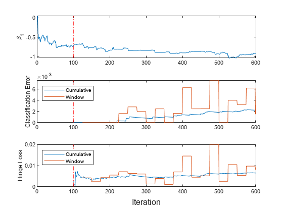
The plot suggests that updateMetricsAndFit does the following:

  • Fit β1 during all incremental learning iterations.

  • Compute the performance metrics after the metrics warm-up period only.

  • Compute the cumulative metrics during each iteration.

  • Compute the window metrics after processing 500 observations (25 iterations).

Input Arguments

collapse all

Traditionally trained linear model or linear model template, specified as a ClassificationLinear model object returned by fitclinear or a template object returned by templateLinear, respectively.

Note

  • The Lambda property of Mdl must be a numeric scalar. If Lambda is a numeric vector for a traditionally trained linear model, you must select the model corresponding to one regularization strength in the regularization path by using selectModels.

  • Incremental learning functions support only numeric input predictor data. If Mdl was trained on categorical data, you must prepare an encoded version of the categorical data to use incremental learning functions. Use dummyvar to convert each categorical variable to a numeric matrix of dummy variables. Then, concatenate all dummy variable matrices and any other numeric predictors, in the same way that the training function encodes categorical data. For more details, see Dummy Variables.

  • If Mdl is a linear model template object, incrementalLearner determines whether to standardize the predictor variables based on the Standardize property of the model template object. For more information, see Standardize Data.

Name-Value Arguments

Specify optional pairs of arguments as Name1=Value1,...,NameN=ValueN, where Name is the argument name and Value is the corresponding value. Name-value arguments must appear after other arguments, but the order of the pairs does not matter.

Before R2021a, use commas to separate each name and value, and enclose Name in quotes.

Example: 'Solver','scale-invariant','MetricsWindowSize',100 specifies the adaptive scale-invariant solver for objective optimization, and specifies processing 100 observations before updating the window performance metrics.

General Options

collapse all

Objective function minimization technique, specified as the comma-separated pair consisting of 'Solver' and a value in this table.

ValueDescriptionNotes
'scale-invariant'

Adaptive scale-invariant solver for incremental learning [1]

  • This algorithm is parameter free and can adapt to differences in predictor scales. Try this algorithm before using SGD or ASGD.

  • To shuffle an incoming chunk of data before the fit function fits the model, set Shuffle to true.

'sgd'Stochastic gradient descent (SGD) [3][2]

  • To train effectively with SGD, standardize the data and specify adequate values for hyperparameters using options listed in SGD and ASGD Solver Options.

  • The fit function always shuffles an incoming chunk of data before fitting the model.

'asgd'Average stochastic gradient descent (ASGD) [4]

  • To train effectively with ASGD, standardize the data and specify adequate values for hyperparameters using options listed in SGD and ASGD Solver Options.

  • The fit function always shuffles an incoming chunk of data before fitting the model.

The default Solver value depends on the input model object Mdl:

  • If Mdl uses ridge regularization and the SGD or ASGD solver, IncrementalMdl uses the same solver.

    (If Mdl is a traditionally trained model, you can view the Solver value in Mdl.ModelParameters.Solver. If Mdl is a model template, you can view the Solver value by displaying the object in the Command Window or the Variables editor.)

  • Otherwise, the default Solver value is 'scale-invariant'.

Example: 'Solver','sgd'

Data Types: char | string

Number of observations processed by the incremental model to estimate hyperparameters before training or tracking performance metrics, specified as the comma-separated pair consisting of 'EstimationPeriod' and a nonnegative integer.

Note

  • If Mdl is prepared for incremental learning (all hyperparameters required for training are specified), incrementalLearner forces EstimationPeriod to 0.

  • If Mdl is not prepared for incremental learning, incrementalLearner sets EstimationPeriod to 1000.

For more details, see Estimation Period.

Example: 'EstimationPeriod',100

Data Types: single | double

SGD and ASGD Solver Options

collapse all

Mini-batch size, specified as the comma-separated pair consisting of 'BatchSize' and a positive integer. At each learning cycle during training, incrementalLearner uses BatchSize observations to compute the subgradient.

The number of observations for the last mini-batch (last learning cycle in each function call of fit or updateMetricsAndFit) can be smaller than BatchSize. For example, if you supply 25 observations to fit or updateMetricsAndFit, the function uses 10 observations for the first two learning cycles and uses 5 observations for the last learning cycle.

The default BatchSize value depends on the input model object Mdl:

  • If Mdl uses ridge regularization and the SGD or ASGD solver, you cannot set BatchSize. Instead, incrementalLearner sets BatchSize to Mdl.ModelParameters.BatchSize of the traditionally trained model, or to the BatchSize property of the model template.

  • Otherwise, the default BatchSize value is 10.

Example: 'BatchSize',1

Data Types: single | double

Ridge (L2) regularization term strength, specified as a nonnegative scalar.

The default Lambda value depends on the input model object Mdl:

  • If Mdl uses ridge regularization and the SGD or ASGD solver, you cannot set Lambda. Instead, incrementalLearner sets Lambda to the Lambda property of Mdl.

  • Otherwise, the default Lambda value is 1e-5.

Note

incrementalLearner does not support lasso regularization. If the Regularization property of Mdl is 'lasso (L1)', incrementalLearner uses ridge regularization instead, and sets the Solver name-value argument to 'scale-invariant' by default.

Example: 'Lambda',0.01

Data Types: single | double

Initial learning rate, specified as 'auto' or a positive scalar.

The learning rate controls the optimization step size by scaling the objective subgradient. LearnRate specifies an initial value for the learning rate, and LearnRateSchedule determines the learning rate for subsequent learning cycles.

When you specify 'auto':

  • The initial learning rate is 0.7.

  • If EstimationPeriod > 0, fit and updateMetricsAndFit change the rate to 1/sqrt(1+max(sum(X.^2,obsDim))) at the end of EstimationPeriod. When the observations are the columns of the predictor data X collected during the estimation period, the obsDim value is 1; otherwise, the value is 2.

The default LearnRate value depends on the input model object Mdl:

  • If Mdl uses ridge regularization and the SGD or ASGD solver, you cannot set LearnRate. Instead, incrementalLearner sets LearnRate to Mdl.ModelParameters.LearnRate of the traditionally trained model, or to the LearnRate property of the model template.

  • Otherwise, the default LearnRate value is 'auto'.

Example: 'LearnRate',0.001

Data Types: single | double | char | string

Learning rate schedule, specified as the comma-separated pair consisting of 'LearnRateSchedule' and a value in this table, where LearnRate specifies the initial learning rate ɣ0.

ValueDescription
'constant'The learning rate is ɣ0 for all learning cycles.
'decaying'

The learning rate at learning cycle t is

γt=γ0(1+λγ0t)c.

  • λ is the value of Lambda.

  • If Solver is 'sgd', then c = 1.

  • If Solver is 'asgd', then c is 0.75 [4].

If Mdl uses ridge regularization and the SGD or ASGD solver, you cannot set LearnRateSchedule. Instead, incrementalLearner sets LearnRateSchedule to 'decaying'.

Example: 'LearnRateSchedule','constant'

Data Types: char | string

Adaptive Scale-Invariant Solver Options

collapse all

Flag for shuffling the observations in the batch at each iteration, specified as the comma-separated pair consisting of 'Shuffle' and a value in this table.

ValueDescription
trueThe software shuffles an incoming chunk of data before the fit function fits the model. This action reduces bias induced by the sampling scheme.
falseThe software processes the data in the order received.

Example: 'Shuffle',false

Data Types: logical

Performance Metrics Options

collapse all

Model performance metrics to track during incremental learning with the updateMetrics or updateMetricsAndFit function, specified as a built-in loss function name, string vector of names, function handle (@metricName), structure array of function handles, or cell vector of names, function handles, or structure arrays.

The following table lists the built-in loss function names. You can specify more than one by using a string vector.

NameDescription
"binodeviance"Binomial deviance
"classiferror"Classification error
"exponential"Exponential loss
"hinge"Hinge loss
"logit"Logistic loss
"quadratic"Quadratic loss

For more details on the built-in loss functions, see loss.

Example: 'Metrics',["classiferror" "hinge"]

To specify a custom function that returns a performance metric, use function handle notation. The function must have this form:

metric = customMetric(C,S)

  • The output argument metric is an n-by-1 numeric vector, where each element is the loss of the corresponding observation in the data processed by the incremental learning functions during a learning cycle.

  • You specify the function name (customMetric).

  • C is an n-by-2 logical matrix with rows indicating the class to which the corresponding observation belongs. The column order corresponds to the class order in the model for incremental learning. Create C by setting C(p,q) = 1, if observation p is in class q, for each observation in the specified data. Set the other element in row p to 0.

  • S is an n-by-2 numeric matrix of predicted classification scores. S is similar to the score output of predict, where rows correspond to observations in the data, and the column order corresponds to the class order in the model for incremental learning. S(p,q) is the classification score of observation p being classified in class q.

To specify multiple custom metrics and assign a custom name to each, use a structure array. To specify a combination of built-in and custom metrics, use a cell vector.

Example: 'Metrics',struct('Metric1',@customMetric1,'Metric2',@customMetric2)

Example: 'Metrics',{@customMetric1 @customMetric2 'logit' struct('Metric3',@customMetric3)}

updateMetrics and updateMetricsAndFit store specified metrics in a table in the property IncrementalMdl.Metrics. The data type of Metrics determines the row names of the table.

'Metrics' Value Data TypeDescription of Metrics Property Row NameExample
String or character vectorName of corresponding built-in metricRow name for "classiferror" is "ClassificationError"
Structure arrayField nameRow name for struct('Metric1',@customMetric1) is "Metric1"
Function handle to function stored in a program fileName of functionRow name for @customMetric is "customMetric"
Anonymous functionCustomMetric_j, where j is metric j in MetricsRow name for @(C,S)customMetric(C,S)... is CustomMetric_1

For more details on performance metrics options, see Performance Metrics.

Data Types: char | string | struct | cell | function_handle

Number of observations the incremental model must be fit to before it tracks performance metrics in its Metrics property, specified as a nonnegative integer. The incremental model is warm after incremental fitting functions fit (EstimationPeriod + MetricsWarmupPeriod) observations to the incremental model.

For more details on performance metrics options, see Performance Metrics.

Example: 'MetricsWarmupPeriod',50

Data Types: single | double

Number of observations to use to compute window performance metrics, specified as a positive integer.

For more details on performance metrics options, see Performance Metrics.

Example: 'MetricsWindowSize',100

Data Types: single | double

Output Arguments

collapse all

Binary classification linear model for incremental learning, returned as an incrementalClassificationLinear model object. IncrementalMdl is also configured to generate predictions given new data (see predict).

To initialize IncrementalMdl for incremental learning, incrementalLearner passes the values of the Mdl properties in this table to corresponding properties of IncrementalMdl.

Input Object Mdl TypePropertyDescription
ClassificationLinear model object or linear model template objectBetaLinear model coefficients, a numeric vector
BiasModel intercept, a numeric scalar
LearnerLinear classification model type, a character vector
ModelParameters.FitBias of a model object or FitBias of a template objectLinear model intercept inclusion flag, a logical scalar
ClassificationLinear model objectClassNamesClass labels for binary classification, a two-element list
NumPredictorsNumber of predictors, a positive integer
PriorPrior class label distribution, a numeric vector
ScoreTransformScore transformation function, a function name or function handle

If Mdl uses ridge regularization and the SGD or ASGD solver, incrementalLearner also passes the properties in this table.

Input Object Mdl TypePropertyDescription
ClassificationLinear model object or linear model template objectLambdaRidge (L2) regularization term strength, a nonnegative scalar
ModelParameters.LearnRate of a model object or LearnRate of a template objectLearning rate, a positive scalar
ModelParameters.BatchSize of a model object or BatchSize of a template objectMini-batch size, a positive integer
ModelParameters.Solver of a model object or Solver of a template objectObjective function minimization technique, a character vector

Note that incrementalLearner does not use the Cost property of the traditionally trained model in Mdl because incrementalClassificationLinear does not support this property.

More About

collapse all

Incremental Learning

Incremental learning, or online learning, is a branch of machine learning concerned with processing incoming data from a data stream, possibly given little to no knowledge of the distribution of the predictor variables, aspects of the prediction or objective function (including tuning parameter values), or whether the observations are labeled. Incremental learning differs from traditional machine learning, where enough labeled data is available to fit to a model, perform cross-validation to tune hyperparameters, and infer the predictor distribution.

Given incoming observations, an incremental learning model processes data in any of the following ways, but usually in this order:

  • Predict labels.

  • Measure the predictive performance.

  • Check for structural breaks or drift in the model.

  • Fit the model to the incoming observations.

For more details, see Incremental Learning Overview.

Adaptive Scale-Invariant Solver for Incremental Learning

The adaptive scale-invariant solver for incremental learning, introduced in [1], is a gradient-descent-based objective solver for training linear predictive models. The solver is hyperparameter free, insensitive to differences in predictor variable scales, and does not require prior knowledge of the distribution of the predictor variables. These characteristics make it well suited to incremental learning.

The standard SGD and ASGD solvers are sensitive to differing scales among the predictor variables, resulting in models that can perform poorly. To achieve better accuracy using SGD and ASGD, you can standardize the predictor data, and tune the regularization and learning rate parameters. For traditional machine learning, enough data is available to enable hyperparameter tuning by cross-validation and predictor standardization. However, for incremental learning, enough data might not be available (for example, observations might be available only one at a time) and the distribution of the predictors might be unknown. These characteristics make parameter tuning and predictor standardization difficult or impossible to do during incremental learning.

The incremental fitting functions for classification fit and updateMetricsAndFit use the more aggressive ScInOL2 version of the algorithm.

Algorithms

collapse all

Estimation Period

During the estimation period, the incremental fitting functions fit and updateMetricsAndFit use the first incoming EstimationPeriod observations to estimate (tune) hyperparameters required for incremental training. Estimation occurs only when EstimationPeriod is positive. This table describes the hyperparameters and when they are estimated, or tuned.

HyperparameterModel PropertyUsageConditions
Predictor means and standard deviations

Mu and Sigma

Standardize predictor data

The hyperparameters are estimated when both of these conditions apply:

  • Incremental fitting functions are configured to standardize predictor data (see Standardize Data).

  • Mdl.Mu and Mdl.Sigma are empty arrays [].

Learning rateLearnRateAdjust the solver step size

The hyperparameter is estimated when both of these conditions apply:

  • You change the solver of Mdl to SGD or ASGD (see Solver).

  • You do not specify the 'LearnRate' name-value argument as a positive scalar.

During the estimation period, fit does not fit the model, and updateMetricsAndFit does not fit the model or update the performance metrics. At the end of the estimation period, the functions update the properties that store the hyperparameters.

Standardize Data

If incremental learning functions are configured to standardize predictor variables, they do so using the means and standard deviations stored in the Mu and Sigma properties of the incremental learning model IncrementalMdl.

  • When you set Standardize=true by using the Standardize name-value argument of templateLinear, and the Mdl.Mu and Mdl.Sigma properties are empty, the following conditions apply:

    • If the estimation period is positive (see the EstimationPeriod property of IncrementalMdl), incremental fitting functions estimate the means and standard deviations using the estimation period observations.

    • If the estimation period is 0, incrementalLearner forces the estimation period to 1000. Consequently, incremental fitting functions estimate new predictor variable means and standard deviations during the forced estimation period.

  • When incremental fitting functions estimate predictor means and standard deviations, the functions compute weighted means and weighted standard deviations using the estimation period observations. Specifically, the functions standardize predictor j (xj) using

    xj=xjμjσj.

    • xj is predictor j, and xjk is observation k of predictor j in the estimation period.

    • μj=1kwkkwkxjk.

    • (σj)2=1kwkkwk(xjkμj)2.

    • wj=wjjClass kwjpk,

      • pk is the prior probability of class k (Prior property of the incremental model).

      • wj is observation weight j.

Performance Metrics

  • The updateMetrics and updateMetricsAndFit functions are incremental learning functions that track model performance metrics ('Metrics') from new data when the incremental model is warm (IsWarm property). An incremental model becomes warm after fit or updateMetricsAndFit fit the incremental model to 'MetricsWarmupPeriod' observations, which is the metrics warm-up period.

    If 'EstimationPeriod' > 0, the functions estimate hyperparameters before fitting the model to data. Therefore, the functions must process an additional EstimationPeriod observations before the model starts the metrics warm-up period.

  • The Metrics property of the incremental model stores two forms of each performance metric as variables (columns) of a table, Cumulative and Window, with individual metrics in rows. When the incremental model is warm, updateMetrics and updateMetricsAndFit update the metrics at the following frequencies:

    • Cumulative — The functions compute cumulative metrics since the start of model performance tracking. The functions update metrics every time you call the functions and base the calculation on the entire supplied data set.

    • Window — The functions compute metrics based on all observations within a window determined by the 'MetricsWindowSize' name-value pair argument. 'MetricsWindowSize' also determines the frequency at which the software updates Window metrics. For example, if MetricsWindowSize is 20, the functions compute metrics based on the last 20 observations in the supplied data (X((end – 20 + 1):end,:) and Y((end – 20 + 1):end)).

      Incremental functions that track performance metrics within a window use the following process:

      1. Store a buffer of length MetricsWindowSize for each specified metric, and store a buffer of observation weights.

      2. Populate elements of the metrics buffer with the model performance based on batches of incoming observations, and store corresponding observation weights in the weights buffer.

      3. When the buffer is filled, overwrite IncrementalMdl.Metrics.Window with the weighted average performance in the metrics window. If the buffer is overfilled when the function processes a batch of observations, the latest incoming MetricsWindowSize observations enter the buffer, and the earliest observations are removed from the buffer. For example, suppose MetricsWindowSize is 20, the metrics buffer has 10 values from a previously processed batch, and 15 values are incoming. To compose the length 20 window, the functions use the measurements from the 15 incoming observations and the latest 5 measurements from the previous batch.

  • The software omits an observation with a NaN score when computing the Cumulative and Window performance metric values.

References

[1] Kempka, Michał, Wojciech Kotłowski, and Manfred K. Warmuth. "Adaptive Scale-Invariant Online Algorithms for Learning Linear Models." Preprint, submitted February 10, 2019. https://arxiv.org/abs/1902.07528.

[2] Langford, J., L. Li, and T. Zhang. “Sparse Online Learning Via Truncated Gradient.” J. Mach. Learn. Res., Vol. 10, 2009, pp. 777–801.

[3] Shalev-Shwartz, S., Y. Singer, and N. Srebro. “Pegasos: Primal Estimated Sub-Gradient Solver for SVM.” Proceedings of the 24th International Conference on Machine Learning, ICML ’07, 2007, pp. 807–814.

[4] Xu, Wei. “Towards Optimal One Pass Large Scale Learning with Averaged Stochastic Gradient Descent.” CoRR, abs/1107.2490, 2011.

Version History

Introduced in R2020b