Specify Custom Signal Objective with Uncertain Variable (GUI)
This example shows how to specify a custom objective function for a model signal. You calculate the objective function value using a variable that models parameter uncertainty.
Competitive Population Dynamics Model
The Simulink® model sdoPopulation models a simple two-organism ecology using the competitive Lotka-Volterra equations:
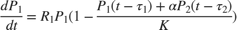
 is the population size of the n-th organism.
 is the inherent per capita growth rate of each organism.
 is the competitive delay for each organism.
 is the carrying capacity of the organism environment.
 is the proximity of the two populations and how strongly they affect each other.
The model uses normalized units.
The two-dimensional signal, P, models the population sizes for P1 (first element) and P2 (second element). The model is initially configured with one organism, P1, dominating the ecology.
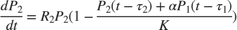
Open the model and simulate its initial response.
open_system("sdoPopulation")
sim("sdoPopulation")
The Population scope shows the P1 population oscillating between high and low values, while P2 is constant at 0.1

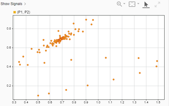
The Population Phase Portrait block shows the population sizes of the two organisms in relation to each other.
Population Stabilization Design Problem
Tune the  ,
,  , and values to meet the following design requirements.
Minimize the population range, that is, the maximum difference between
P1andP2.
Stabilize
P1andP2, that is, ensure that neither organism population dies off or grows extremely large.
You must tune the parameters for different values of the carrying capacity, . This ensures robustness to environment carrying-capacity uncertainty.
Open Response Optimizer
Double-click the Open Optimization Tool block in the model to open a pre-configured Response Optimizer session. The session specifies the following variables:
DesignVars- Design variables set for the, , and model parameters.
K_unc- Uncertain parameter modeling the carrying capacity of the organism environment (). K_uncspecifies the nominal value and two sample values.
P1andP2- Logged signals representing the populations of the two organisms.
Specify Custom Signal Objective Function
Specify a custom requirement to minimize the maximum difference between the two population sizes. Apply this requirement to the P1 and P2 model signals.
Open the Create Requirement dialog box. In the New list, select Custom Requirement.
Specify the following in the Create Requirement dialog box:
Name - Enter
PopulationRange.Type - Select Minimize the function output from the list.
Function - Enter
@sdoPopulation_PopRange. For more information about this function, see Custom Signal Objective Function Details.Select Signals and Systems to Bound (Optional) - Select the
P1andP2check boxes.
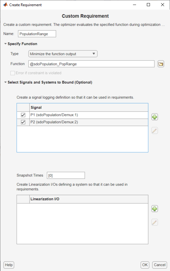
3. Click OK.
A new variable, PopulationRange, appears in the Response Optimizer browser.
Custom Signal Objective Function Details
PopulationRange uses the sdoPopulation_PopRange function. This function computes the maximum difference between the populations, across different environment carrying capacity values. By minimizing this value, you can achieve both design goals. The function is called by the optimizer at each iteration step.
To view the function, type edit sdoPopulation_PopRange. The following discusses details of this function.
Input/Output
The function accepts data, a structure with the following fields:
DesignVars- Current iteration values of, , and .
Nominal- Logged signal data, obtained by simulating the model using parameter values specified bydata.DesignVarsand nominal values for all other parameters. TheNominalfield is itself a structure with fields for each logged signal. The field names are the logged signal names. The custom requirement uses the logged signals,P1andP2. Therefore,data.Nominal.P1anddata.Nominal.P2are timeseries objects corresponding toP1andP2.
Uncertain- Logged signal data, obtained by simulating the model using the sample values of the uncertain variableK_unc. TheUncertainfield is a vector ofNstructures, whereNis the number of sample values specified forK_unc. Each element of this vector is similar todata.Nominaland contains simulation results obtained from a corresponding sample value specified forK_unc.
The function returns the maximum difference between the population sizes across different carrying capacities. The following code snippet in the function performs this action:
val = max(maxP(1)-minP(2),maxP(2)-minP(1));
Data Time Range
When computing the design goals, discard the initial population growth data to eliminate biases from the initial-condition. The following code snippet in the function performs this action:
%Get the population data
tMin = 5; %Ignore signal values prior to this time
iTime = data.Nominal.P1.Time > tMin;
sigData = [data.Nominal.P1.Data(iTime), data.Nominal.P2.Data(iTime)];
iTime represents the time interval of interest, and the columns of sigData contain P1 and P2 data for this interval.
Optimization for Different Values of Carrying Capacity
The function includes the effects of varying the carrying capacity by iterating through the elements of data.Uncertain. The following code snippet in the function performs this action:
...
for ct=1:numel(data.Uncertain)
   iTime = data.Uncertain(ct).P1.Time > tMin;
   sigData = [data.Uncertain(ct).P1.Data(iTime), data.Uncertain(ct).P2.Data(iTime)];
   maxP = max([maxP; max(sigData)]);  %Update maximum if new signals are bigger
   minP = min([minP; min(sigData)]);  %Update minimum if new signals are smaller
end
...
The maximum and minimal populations are obtained across all the simulations contained in data.Uncertain.
Optimize Design
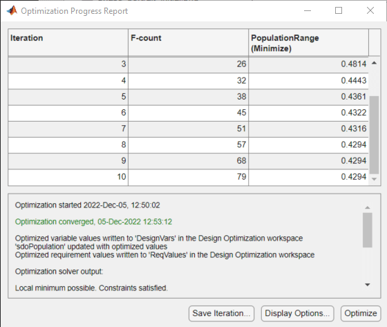
Click Optimize.
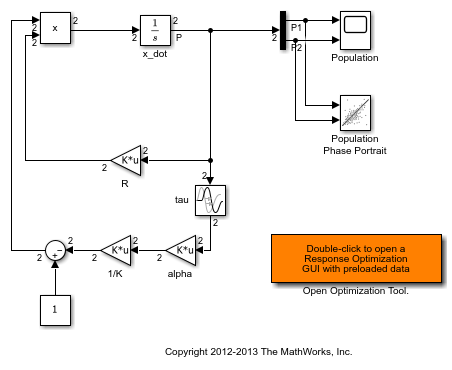
The optimization converges after a number of iterations.
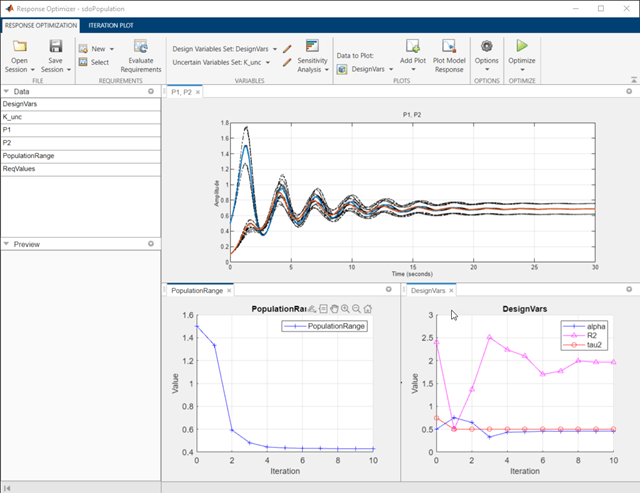
The P1,P2 plot shows the population dynamics, with the first organism population in blue and the second organism population in red. The dotted lines indicate the population dynamics for different environment capacity values. The PopulationRange plot shows that the maximum difference between the two organism populations reduces over time.
Simulate the model with the optimized parameters.
The Population Phase Portrait block shows the populations initially varying, but they eventually converge to stable population sizes.
You can also see this result in the |Population| scope.
