Set Model to Steady-State When Estimating Parameters (Code)
This example shows how to set a model to steady-state in the process of parameter estimation. Setting a model to steady-state is important in many applications such as power systems and aircraft dynamics. This example uses a population dynamics model.
This example requires Simulink® Control Design™ software.
Model Description
The Simulink model sdoPopulationInflux models a simple ecology where an organism population growth is limited by the carrying capacity of the environment.
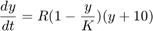
 is the inherent growth rate of the organism population.
 is the carrying capacity of the environment.
There is also an influx of other members of the organism from a neighboring environment. The model uses normalized units.
Open the model.
modelName = 'sdoPopulationInflux';
open_system(modelName)
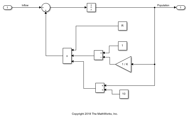
The file sdoPopulationInflux_Data.mat contains data of the population in the environment as well as the influx of additional organisms from the neighboring environment.
load sdoPopulationInflux_Data.mat;   % Time series:  Population_ts  Inflow_ts
hFig = figure;
subplot(2,1,1);
plot(Population_ts)
subplot(2,1,2);
plot(Inflow_ts)
The population starts in a steady state. After some time, there is an influx of organisms from the neighboring environment. Based on the measured data, you can estimate values for the model parameters.
The parameter R represents the inherent growth rate of the organism. Use 1 as the initial guess for this parameter. It is non-negative.
R = sdo.getParameterFromModel(modelName, 'R');
R.Value = 1;
R.Minimum = 0;
The parameter K represents the carrying capacity of the environment. Use 2 as the initial guess for this parameter. It is known to be at least 0.1.
K = sdo.getParameterFromModel(modelName, 'K');
K.Value = 2;
K.Minimum = 0.1;
Collect these parameters into a vector.
v = [R K];
Compare Measured Data to Initial Simulated Output
Create an Experiment object.
Exp = sdo.Experiment(modelName);
Associate Population_ts with model output.
Population = Simulink.SimulationData.Signal;
Population.Name = 'Population';
Population.BlockPath = [modelName  '/Integrator'];
Population.PortType = 'outport';
Population.PortIndex = 1;
Population.Values = Population_ts;
Add Population to the experiment.
Exp.OutputData = Population;
Associate Inflow_ts with model input.
Inflow = Simulink.SimulationData.Signal;
Inflow.Name = 'Population';
Inflow.BlockPath = [modelName  '/In1'];
Inflow.PortType = 'outport';
Inflow.PortIndex = 1;
Inflow.Values = Inflow_ts;
Add Inflow to the experiment.
Exp.InputData = Inflow;
Create a simulation scenario using the experiment, and obtain the simulated output.
Exp = setEstimatedValues(Exp, v);   % use vector of parameters/states
Simulator = createSimulator(Exp);
Simulator = sim(Simulator);
Search for the model output signal in the logged simulation data.
SimLog = find(Simulator.LoggedData,  ...
	get_param(modelName, 'SignalLoggingName') );
PopulationSim = find(SimLog, 'Population');
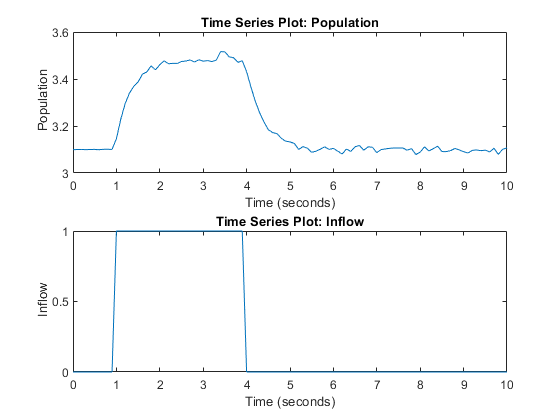
The model output does not match the data very well, indicating a need to compute better estimates of the model parameters.
clf;
plot(PopulationSim.Values, 'r');
hold on;
plot(Population_ts, 'b');
legend('Model Simulation', 'Measured Data',  'Location', 'best');
Estimate Parameters
To estimate parameters, define an objective function to compute the sum squared error between model simulation and measured data.
estFcn = @(v) sdoPopulationInflux_Objective(v, Simulator, Exp);
type sdoPopulationInflux_Objective.m
function vals = sdoPopulationInflux_Objective(v, Simulator, Exp, OpPointSetup)
% Compare model output with data
%
%    Inputs:
%       v            - vector of parameters and/or states
%       Simulator    - used to simulate the model
%       Exp          - Experiment object
%       OpPointSetup - Object to set up computation of steady-state
%                      operating point

% Copyright 2018 The MathWorks, Inc.

%Parse inputs
if nargin < 4
    OpPointSetup = [];
end

% Requirement setup
req = sdo.requirements.SignalTracking;
req.Type = '==';
req.Method = 'Residuals';

% Simulate the model
Exp = setEstimatedValues(Exp, v);   % use vector of parameters/states
Simulator = createSimulator(Exp,Simulator);
strOT = mat2str(Exp.OutputData(1).Values.Time);
if isempty(OpPointSetup)
    Simulator = sim(Simulator, 'OutputOption', 'AdditionalOutputTimes', 'OutputTimes', strOT);
else
    Simulator = sim(Simulator, 'OutputOption', 'AdditionalOutputTimes', 'OutputTimes', strOT, ...
        'OperatingPointSetup', OpPointSetup);
end

% Compare model output with data
SimLog = find(Simulator.LoggedData,  ...
	get_param(Exp.ModelName, 'SignalLoggingName') );
OutputModel = find(SimLog, 'Population');
Model_Error = evalRequirement(req, OutputModel.Values, Exp.OutputData.Values);
vals.F = Model_Error;
%Define options for the optimization.
%
opts = sdo.OptimizeOptions;
opts.Method = 'lsqnonlin';
Estimate the parameters.
vOpt = sdo.optimize(estFcn, v, opts);
disp(vOpt)
 Optimization started 2026-Apr-19, 07:10:57

                                          First-order
 Iter F-count        f(x)      Step-size  optimality
    0      5       12.485            1
    1     10      1.09824        1.184        0.244
    2     15       0.9873        1.088       0.0259
    3     20     0.952948        1.217      0.00624
    4     25     0.946892       0.9151      0.00197
    5     30     0.946484       0.3541      0.00153
Local minimum possible.

lsqnonlin stopped because the final change in the sum of squares relative to
its initial value is less than the value of the function tolerance.

(1,1) =

       Name: 'R'
      Value: 5.5942
    Minimum: 0
    Maximum: Inf
       Free: 1
      Scale: 1
       Info: [1×1 struct]


(1,2) =

       Name: 'K'
      Value: 3.2061
    Minimum: 0.1000
    Maximum: Inf
       Free: 1
      Scale: 2
       Info: [1×1 struct]


1x2 param.Continuous
Use the estimated parameter values in the model, and obtain the model response. Search for the model output signal in the logged simulation data.
Exp = setEstimatedValues(Exp, vOpt);
Simulator = createSimulator(Exp,Simulator);
Simulator = sim(Simulator);
SimLog = find(Simulator.LoggedData,  ...
	get_param(modelName, 'SignalLoggingName') );
PopulationSim = find(SimLog, 'Population');
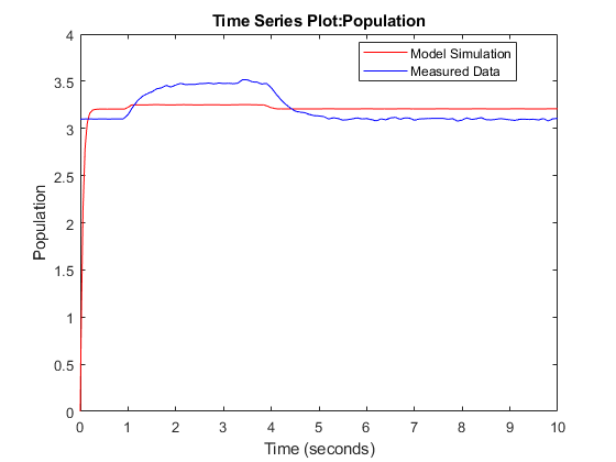
Comparing the measured population data with the optimized model response shows that they still do not match well. There is a transient at the beginning of the model response, where it is markedly different from the measured data.
clf;
plot(PopulationSim.Values, 'r');
hold on;
plot(Population_ts, 'b');
legend('Model Simulation', 'Measured Data',  'Location', 'best');
Put Model in Steady-State During Estimation
To improve the fit between the model and measured data, the model needs to be set to steady-state when parameters are estimated. Define an operating point specification. The input is known from experimental data. Therefore, (1) it should not be treated as a free variable when computing the steady-state operating point, and (2) after the operating point is found, its input should not be used when simulating the model. On the other hand, all the states found when computing the operating point should be used when simulating the model. Create an sdo.OperatingPointSetup object to collect the operating point specification, inputs to use, and states to use, so this information can be passed to the objective function and used when simulating the model. You can also provide a fourth argument to sdo.OperatingPointSetup to specify options for computing the operating point. For example, the option 'graddescent-proj' is often used to find the operating point for systems that use physical modeling.
opSpec = operspec(modelName);
opSpec.Inputs(1).Known = true;
inputsToUse = [];
statesToUse = 1:numel(opSpec.States);
OpPointSetup = sdo.OperatingPointSetup(opSpec, inputsToUse, statesToUse);
Estimate the parameters, setting the model to steady-state in the process.
estFcn = @(v) sdoPopulationInflux_Objective(v, Simulator, Exp, OpPointSetup);
vOpt = sdo.optimize(estFcn, v, opts);
disp(vOpt)
 Optimization started 2026-Apr-19, 07:11:09

                                          First-order
 Iter F-count        f(x)      Step-size  optimality
    0      5      11.1517            1
    1     10     0.025674       0.5732        0.045
    2     15   0.00239293       0.3451        0.357
    3     20  0.000692478       0.0148      0.00301
    4     25   0.00069236    6.539e-05     1.16e-07
Local minimum found.

Optimization completed because the size of the gradient is less than
the value of the optimality tolerance.

(1,1) =

       Name: 'R'
      Value: 0.5953
    Minimum: 0
    Maximum: Inf
       Free: 1
      Scale: 1
       Info: [1×1 struct]


(1,2) =

       Name: 'K'
      Value: 3.0988
    Minimum: 0.1000
    Maximum: Inf
       Free: 1
      Scale: 2
       Info: [1×1 struct]


1x2 param.Continuous
Use the estimated parameter values in the model, and obtain the model response. Search for the model output signal in the logged simulation data.
Exp = setEstimatedValues(Exp, vOpt);
Simulator = createSimulator(Exp,Simulator);
Simulator = sim(Simulator, 'OperatingPointSetup', OpPointSetup);
SimLog = find(Simulator.LoggedData,  ...
	get_param(modelName, 'SignalLoggingName') );
PopulationSim = find(SimLog, 'Population');
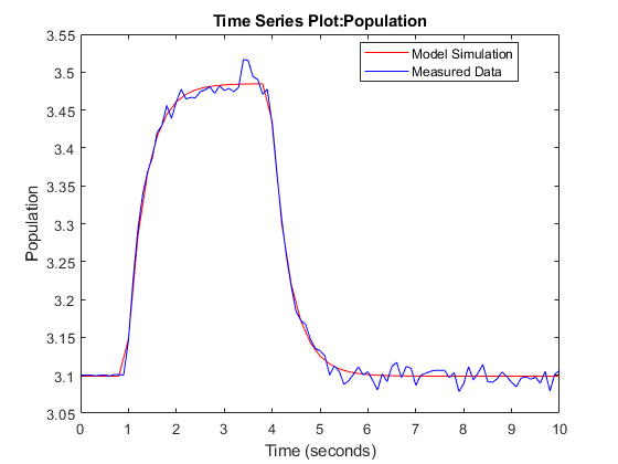
There is no more transient at the beginning of the model response, and there is a much better match between the model response and measured data, which is also reflected by the lower objective/cost function value in the second optimization. All these indicate that a good set of parameter values was found.
clf;
plot(PopulationSim.Values, 'r');
hold on;
plot(Population_ts, 'b');
legend('Model Simulation', 'Measured Data',  'Location', 'best');
Related Examples
To learn how to put models in a steady state using the Parameter Estimator app, see Set Model to Steady-State When Estimating Parameters (GUI).
Close the model and figure.
bdclose(modelName)
close(hFig)