Engine Design and Cost Tradeoffs

Open Script

This example shows how to use Simulink® Design Optimization™ to optimize a design for performance and cost. In this example, you tune an automotive engine speed controller while reducing controller costs by tuning sensor accuracy and actuator response time.

Opening the Model

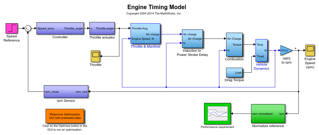
Open the automotive engine model using the command below. The following subsystems model the engine response: Throttle & Manifold, Induction to Power Stroke Delay, Combustion, Drag Torque and Vehicle Dynamics. The main signal of interest in the model is the engine speed in rpm. The control system consists of the lead-lag Controller, rpm Sensor, and Throttle actuator blocks. The model is driven by a step change in speed reference.

open_system('enginetradeoff_demo')

Design Overview

The design has the following objectives:

Engine performance objective:

The engine must respond to step changes in the speed reference with the following characteristics:

Maximum overshoot of 2%

Rise time of 4 seconds to reach 90% of the reference speed

Settling time of 7.5 seconds to reach within 2% of the reference speed

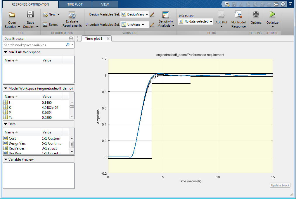
This objective is included as a constraint in the Performance requirement block. The input to this block is the engine speed, which is normalized by the speed reference value. This means that although the speed reference changes, the performance requirement remains the same.

Cost minimization objective:

The design cost of the controller is to be minimized. This objective uses sensor and actuator parameterization to compute a design cost. The design cost is computed so that it is always greater than 1 and the optimization attempts to drive the cost to 1.

We use a custom requirement to minimize this cost. The enginetradeoff_cost function used by the custom requirement simply returns the cost value to be minimized.

type enginetradeoff_cost

function Cost = enginetradeoff_cost(u)
%Compute controller cost based on sensor accuracy, actuator response, and
%controller sampling time.

% Copyright 2013 The MathWorks, Inc.

%Cost constants
min_cost       = 1;       %Minimum cost > 0
sensor_var_min = 1e-3;    %Minimum sensor variance (most expensive)
sampling_min   = 1e-2;    %Minimum controller sampling time (most expensive)
throttle_max   = 2*pi*10; %Maximum actuator response frequency (most expensive)

%Get variable names
varnames = {u.DesignVars.Name};

%Form cost
Cost = min_cost;
%Add sensor cost
index = strcmp(varnames, 'sensor_std');
if any(index)
  Cost = Cost + sensor_var_min./max(u.DesignVars(index).Value,sensor_var_min);
end

%Add sampling cost
index = strcmp(varnames, 'Ts');
if any(index)
  Cost = Cost+ sampling_min./max(u.DesignVars(index).Value,sampling_min);
end

%Add throttle cost
index = strcmp(varnames, 'Tthrottle');
if any(index)
  Cost = Cost + u.DesignVars(index).Value/throttle_max;
end

Model parameterization:

To achieve the performance and cost objectives, we parameterize the following in the model:

Final step value of the speed reference: This ensures that the design works over a range of operating points, from low speed to high speed values.

Gain, pole and zero values of the controller: This allows us to change the controller performance. We tune these values using optimization.

Response time of the throttle actuator: The response time is optimized to minimize controller cost. The actuator cost is inversely proportional to the response time, i.e., a faster response time implies a more expensive actuator.

Accuracy of the rpm sensor: The accuracy is specified by a standard deviation value and optimized to minimize controller cost. The sensor cost is inversely proportional to standard deviation, i.e., a smaller standard deviation implies a more accurate sensor, which is more expensive.

Running the Optimization

Optimizing the engine controller for performance and cost involves:

Optimizing the controller, sensor, and actuator parameters.

Optimizing the response over different operating conditions.

With problems of this type, it is a good practice to build the design iteratively rather than optimizing for all objectives together. Here, we use the divide and conquer strategy as shown in the table below. The idea is to use the optimized parameter values from one stage as the initial guess for the next stage.

You can launch the Response Optimizer using the Apps menu in the Simulink toolstrip, or the sdotool command in MATLAB®. You can launch a pre-configured optimization task in the Response Optimizer by first opening the model and by double-clicking on the orange block at the bottom of the model. From the Response Optimizer, press the Plot Model Response button to simulate the model and show how well the initial design satisfies the design requirements.

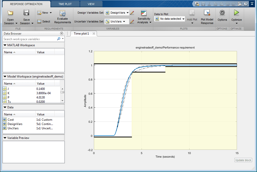
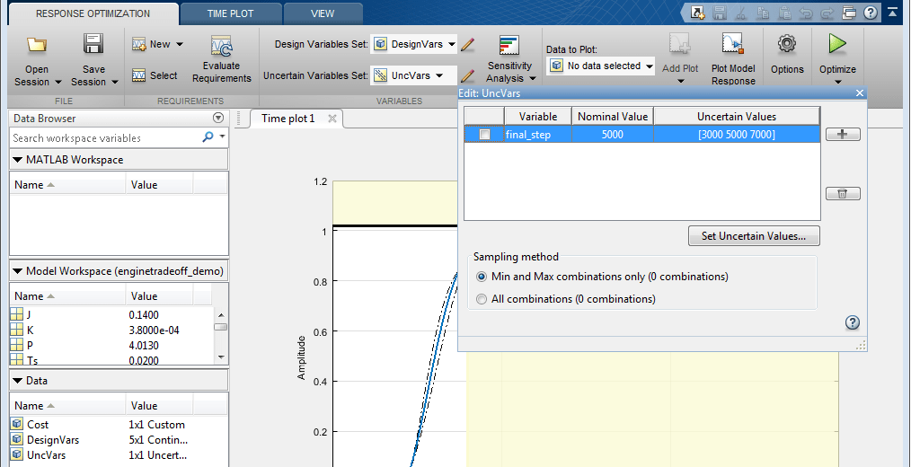
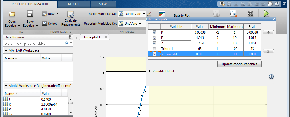
The optimization project saved with the example corresponds to stage 2. In this stage, we optimize the controller parameters over the operating range. To do so, we specify K, P and Z as tuned parameters and the final step value, final_step, of the reference signal as an uncertain parameter. At this stage, the custom controller cost objective is not included in the optimization problem.

We introduce the controller cost objective in stage 3 by configuring the model as follows:

Open the Uncertain Variables editor from the Response Optimizer and then clear the check box for final_step. This removes sweeping the model over different operating points from the optimization problem and thus reduces computational load.

Open the Design Variables editor from the Response Optimizer and then select the check box for sensor_std to tune this parameter.

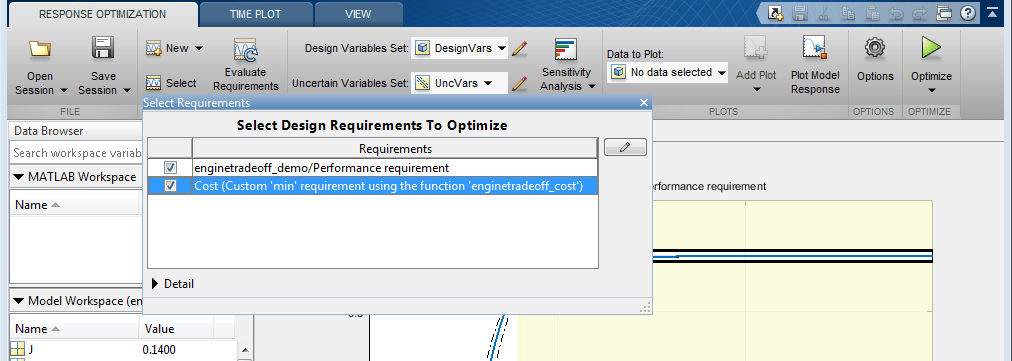
Click the Select button in the Response Optimizer to open the Design Requirements editor, and then select the check box for custom Cost. This accounts for the cost minimization objective during optimization.

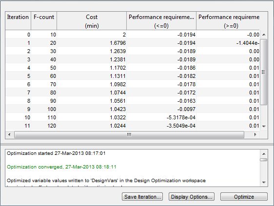
We start the optimization by pressing the Optimize button from the Response Optimizer. The plots are updated to indicate that the design requirements are now satisfied.

To configure the optimization for Stage 4:

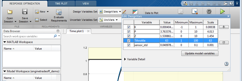
Open the Design Variables editor from the Response Optimizer and then select the check box for Tthrottle to tune this parameter.

You can start the optimization by pressing the Optimize button from Response Optimizer.

To configure the optimization for stage 5:

Open the Uncertain Variables editor from the Response Optimizer and then select the check box for final_step to sweep the model over the operating range.

You can start the optimization by pressing the Optimize button from the Response Optimizer.

% Close the model.
bdclose('enginetradeoff_demo')