Design Optimization to Meet Frequency-Domain Requirements (Code)
This example shows how to tune model parameters to meet frequency-domain requirements, using the sdo.optimize command.
This example requires Simulink® Control Design™.
Suspension Model
Open the Simulink model.
open_system('sdoSimpleSuspension')

Mass-spring-damper models represent simple suspension systems and for this example we tune the system to meet typical suspension requirements. The model implements the second order system representing a mass-spring-damper using Simulink blocks and includes:
a
Massgain block parameterized by the total suspended mass,m0+mLoad. The total mass is the sum of a nominal mass,m0, and a variable load mass,mLoad.
a
Dampergain block parameterized by the damping coefficient,b.
a
Springgain block parameterized by the spring constant,k.
two integrator blocks to compute the mass velocity and position.
a
Band-Limited Disturbance Forceblock applying a disturbance force to the mass. The disturbance force is assumed to be band-limited white noise.
Simulate the model to view the system response to the applied disturbance force.
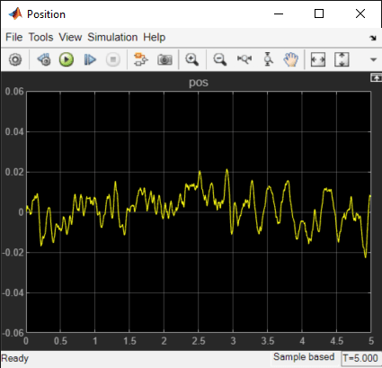
Design Problem
The initial system has a bandwidth that is too high. This can be seen from the spiky position signal. You tune the spring and damper values to meet the following requirements:
The -3dB system bandwidth must not exceed 10 rad/s.
The damping ratio of the system must be less than 1/sqrt(2). This ensures that no frequencies in pass band are amplified by the system.
Minimize the expected failure rate of the system. The expected failure rate is described by a Weibull distribution dependent on the mass, spring, and damper values.
These requirements must all be satisfied as the load mass ranges from 0 to 20 kg.
Specify Design Variables
DesignVars = sdo.getParameterFromModel('sdoSimpleSuspension',{'b','k'});
DesignVars(1).Minimum = 100;
DesignVars(1).Maximum = 10000;
DesignVars(2).Minimum = 10000;
DesignVars(2).Maximum = 100000;
Specify Uncertain Variables
Specify mLoad, the load mass, as an uncertain variable. This will ensure the optimal solution is robust to variations in load mass.
UncVars = sdo.getParameterFromModel('sdoSimpleSuspension','mLoad');
UncVars_Values = {...
    10; ...
    20};
Specify Design Requirements
Specify design requirements to satisfy during optimization.
Requirements = struct;
Requirements.Bandwidth = sdo.requirements.BodeMagnitude(...
    'BoundFrequencies', [10 100], ...
    'BoundMagnitudes', [-3 -3]);
Requirements.DampingRatio = sdo.requirements.PZDampingRatio;
The reliability requirement will be specified in the optimization objective function described below. The reliability requirement is used to tune the spring and damper values to minimize the expected failure rate over a lifetime of 100e3 miles. The failure rate is computed using a Weibull distribution on the damping ratio of the system. As the damping ratio increases, the failure rate is expected to increase.
Linearization Definition
The design requirements use the bandwidth and damping ratio of the system, these frequency domain characteristics require linearizing the model. Create a simulator for the model and use the simulator to compute the linear systems used by the requirements.
Simulator = sdo.SimulationTest('sdoSimpleSuspension');
Specify linear systems to compute by specifying the linearization inputs and outputs of the system. The linear system input is the output of the Band-Limited Disturbance Force block and the linear system output is the output of the x_dot block (the position signal).
IOs(1) = linio('sdoSimpleSuspension/Band-Limited  Disturbance Force',1,'input');
IOs(2) = linio('sdoSimpleSuspension/x_dot',1,'output');
Add the linearization IOs to a sdo.SystemLoggingInfo object with a logging name, and linearization snapshot time. In this case, the snapshot time is set to 0, the model initial condition.
sys1 = sdo.SystemLoggingInfo;
sys1.Source = 'IOs';
sys1.LoggingName = 'IOs';
sys1.LinearizationIOs = IOs;
sys1.SnapshotTimes = 0;
Add the system logging info to the simulator. When the simulator is used to run the model, the linear system defined by the specified linearization IOs is computed and added to the simulation log with the specified logging name.
Simulator.SystemLoggingInfo = sys1;
Create Optimization Objective Function
Create a function that is called at each optimization iteration to evaluate the design requirements.
Use an anonymous function with one argument that calls sdoSimpleSuspension_Design. The sdoSimpleSuspension_Design function has arguments for the design parameters, the simulator, the design requirements, the uncertain variables, and uncertain variable values.
optimfcn = @(P) sdoSimpleSuspension_Design(P,Simulator,Requirements,UncVars,UncVars_Values);
type sdoSimpleSuspension_Design
function Vals = sdoSimpleSuspension_Design(P,Simulator,Requirements,UncVars,UncVars_Values)
%SDOSIMPLESUSPENSION_DESIGN
%
%    The sdoSimpleSuspension_Design function is used to evaluate a simple
%    suspension system design.
%
%    The |P| input argument is the vector of suspension design parameters.
%
%    The |Simulator| input argument is a sdo.SimulinkTest object used to
%    simulate the |sdoSimpleSuspension| model and log simulation signals.
%
%    The |Requirements| input argument contains the design requirements
%    used to evaluate the suspension design.
%
%    The |UncVars| and |UncVars_Values| arguments specify the uncertain
%    variable and uncertain variable values.
%
%    The |Vals| return argument contains information about the design
%    evaluation that can be used by the |sdo.optimize| function to optimize
%    the design.
%
% See also sdoSimpleSuspension_cmddemo

% Copyright 2015 The MathWorks, Inc.

%% Evaluate the suspension reliability
%
%Get the spring and damper design values
allVarNames = {P.Name};
idx         = strcmp(allVarNames,'k');
k           = P(idx).Value;
idx         = strcmp(allVarNames,'b');
b           = P(idx).Value;

%Get the nominal mass from the model workspace
wksp = get_param('sdoSimpleSuspension','ModelWorkspace');
m    = evalin(wksp,'m0');

%The expected failure rate is defined by the Weibull cumulative
%distribution function, 1-exp(-(x/l)^k), where k=3, l is a function of the
%mass, spring and damper values, and x the lifetime.
d        = b/2/sqrt(m*k);
pFailure = 1-exp(-(100e3*d/250e3)^3);

%% Nominal Evaluation
%
% Evaluate the model and requirements with uncertain parameters set to their
% nominal values.

% Simulate the model.
Simulator.Parameters = [P(:);UncVars(:)];
Simulator = sim(Simulator);

% Retrieve logged linearizations.
Sys = find(Simulator.LoggedData,'IOs');

% Evaluate the design requirements.
Cleq_Bandwidth = evalRequirement(Requirements.Bandwidth,Sys.values);
Cleq_DampingRatio = evalRequirement(Requirements.DampingRatio,Sys.values);

%% Uncertain Evaluation
%
% Evaluate the model and requirements for all combinations of uncertain
% parameter values.
for ct=1:size(UncVars_Values,1)
    UncVars(1).Value = UncVars_Values{ct,1};

    % Simulate the model.
    Simulator.Parameters = [P(:);UncVars(:)];
    Simulator = sim(Simulator);

    % Retrieve logged linearizations.
    Sys = find(Simulator.LoggedData,'IOs');

    % Evaluate the design requirements.
    Cleq_Bandwidth_UncVars = evalRequirement(Requirements.Bandwidth,Sys.values);
    Cleq_DampingRatio_UncVars = evalRequirement(Requirements.DampingRatio,Sys.values);

    Cleq_Bandwidth = [Cleq_Bandwidth; Cleq_Bandwidth_UncVars]; %#ok<AGROW>
    Cleq_DampingRatio = [Cleq_DampingRatio; Cleq_DampingRatio_UncVars]; %#ok<AGROW>
end

%% Return Values.
%
% Collect the evaluated design requirement values in a structure to
% return to the optimization solver.
Vals.F = pFailure;
Vals.Cleq = [...
    Cleq_Bandwidth(:); ...
    Cleq_DampingRatio(:)];
end
Optimization Options
Specify optimization options.
Options = sdo.OptimizeOptions;
Options.MethodOptions.Algorithm = 'active-set';
Options.MethodOptions.TolGradCon = 1e-06;
Optimize the Design
Call sdo.optimize with the objective function handle, parameters to optimize, and options.
[Optimized_DesignVars,Info] = sdo.optimize(optimfcn,DesignVars,Options);
 Optimization started 2026-Apr-19, 06:52:04

                               max                     First-order
 Iter F-count        f(x)   constraint    Step-size    optimality
    0      5    0.0619897       0.7642
    1     10     0.351266            0        0.461         1.22
    2     15     0.189345            0        0.188        0.312
    3     20    0.0829063      0.01312         0.51        0.425
    4     24    0.0365398            0        0.308         1.55
    5     28    0.0294977            0       0.0143        0.733
    6     32    0.0293065            0     0.000417      0.00142
Local minimum found that satisfies the constraints.

Optimization completed because the objective function is non-decreasing in
feasible directions, to within the value of the optimality tolerance,
and constraints are satisfied to within the  value of the constraint tolerance.
Related Examples
To learn how to optimize the suspension system using the Response Optimizer, see Design Optimization to Meet Frequency-Domain Requirements (GUI).
Close the model.
bdclose('sdoSimpleSuspension')