Improving Optimization Performance Using Parallel Computing
This example shows how to improve optimization performance using the Parallel Computing Toolbox™. The example discusses the speedup seen when using parallel computing to optimize a complex Simulink® model. The example also shows the effect of the number of parameters and the model simulation time when using parallel computing.
Requires Parallel Computing Toolbox™
An Example Illustrating Optimization Speedup
The main computational load when using Simulink Design Optimization™ is the simulation of a model. The optimization methods typically require numerous simulations per optimization iteration. As many of the simulations are independent, it is beneficial to use parallel computing to distribute these independent simulations across different processors.
Consider the Simulink model of an HL20 aircraft, which ships with the Aerospace Blockset™. The HL20 model is a complex model and includes mechanical, electrical, avionics, and environmental components. A typical simulation of the HL20 model takes around 60 seconds.
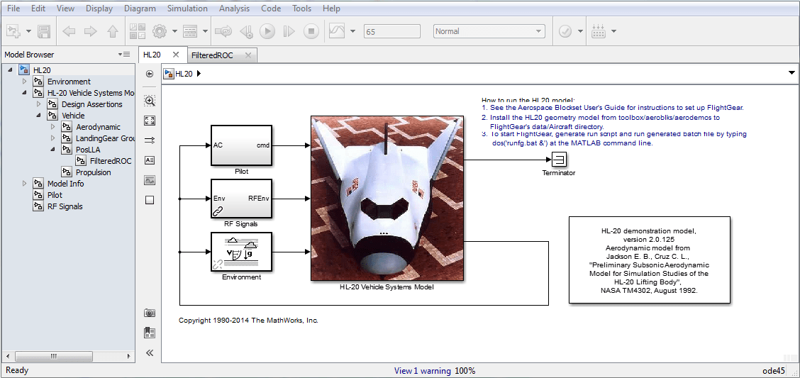
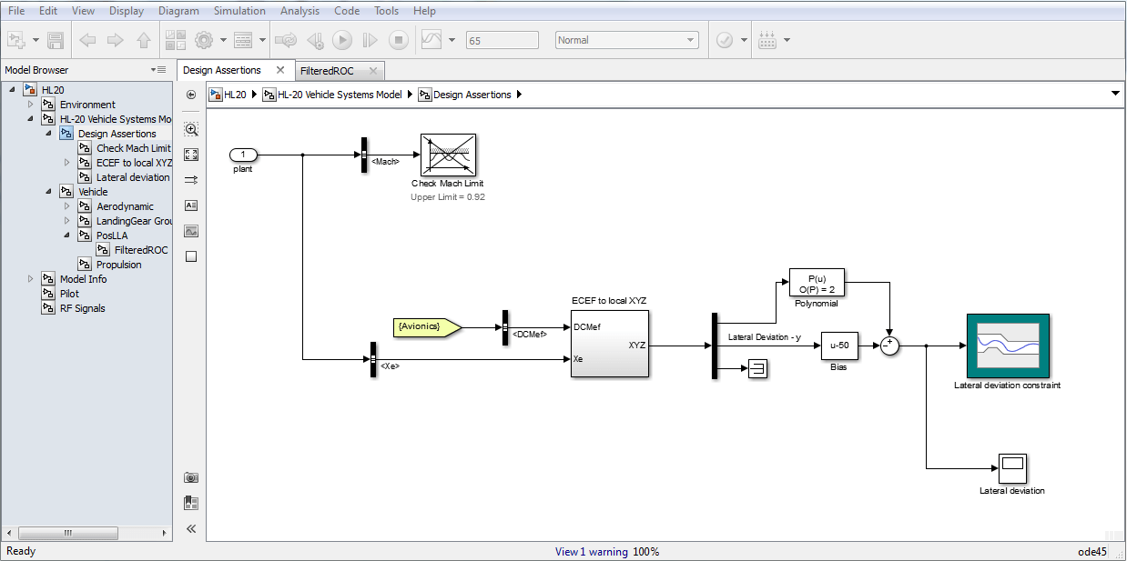
During landing, the aircraft is subjected to two wind gusts from different directions which cause the aircraft to deviate from the nominal trajectory on the runway. Simulink Design Optimization is used to tune the 3 parameters of the controller so that the lateral deviation of the aircraft from a nominal trajectory in the presence of wind gusts is kept within five meters.
The optimization is performed both with and without using parallel computing on dual-core 64bit AMD®, 2.4GHz, 3.4GB Linux® and quad-core 64bit AMD, 2.5GHz, 7.4GB Linux machines. The speed up observed for this problem is shown below.
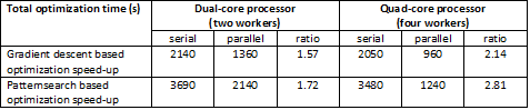
The HL20 example illustrates the potential speedup when using parallel computing. The next sections discuss the speedup expected for other optimization problems.
When Will an Optimization Benefit from Parallel Computing?
The previous section shows that distributing the simulations during an optimization can reduce the total optimization time. This section quantifies the expected speedup.
In general, the following factors could indicate that parallel computing would result in faster optimization:
There are a large number of parameters being optimized
A pattern search method is being used
A complex Simulink model that takes a long time to simulate
There are a number of uncertain parameters in the model
Each of these is examined in the following sections.
Number of Parameters and Their Effect on Parallel Computing
The number of simulations performed by an optimization method is closely coupled with the number of parameters.
Gradient Descent Method and Parallel Computing
Consider the simulations required by a gradient-based optimization method at each iteration:
A simulation for the current solution point
Simulations to compute the gradient of the objective with respect to the optimized parameters
Once a gradient is computed, simulations to evaluate the objective along the direction of the gradient (the so called line search evaluations)
Of these simulations, the simulations required to compute gradients are independent and are distributed. Let us look at this more closely:
Np  = 1:16;   %Number of parameters (16 = 4 filtered PID controllers)
Nls = 1;      %Number of line search simulations, assume 1 for now
Nss = 1;      %Total number of serial simulations, start with nominal only
The gradients are computed using central differences. There are 2 simulations per parameter, and include the line search simulations to give the total number of simulations per iteration:
Nss = 1+Np*2+Nls;
As mentioned above, the computation of gradients with respect to each parameter can be distributed or run in parallel. This reduces the total number of simulations that run in series when using parallel computing as follows:
Nw  = 4;      %Number of parallel processors
Nps = 1 + ceil(Np/Nw)*2+Nls;
The ratio Nss/Nps gives us the speedup which we plot below
Nls = 0:5;      %Vary the number of line search simulations
figure;
hAx  = gca;
xlim([min(Np) max(Np)]);
for ct = 1:numel(Nls)
  Rf = (1+Nls(ct)+Np*2)./(1+Nls(ct)+ceil(Np/Nw)*2);
  hLine = line('parent',hAx,'xdata',Np,'ydata',Rf);
  if ct == 1
     hLine.LineStyle = '-';
     hLine.Color = [0 0 1];
     hLine.LineWidth = 1;
  else
     hLine.LineStyle = '-.';
     hLine.Color = [0.6 0.6 1];
     hLine.LineWidth = 1;
  end
end
grid on
title('Gradient descent based relative speedup')
xlabel('Number of parameters')
ylabel('Serial time/parallel time')
annotation('arrow',[0.55 .55],[5/6 2/6])
text(8.5,1.75,'Increasing number of line searches')
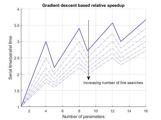
The plot shows that the relative speedup gets better as more parameters are added. The upper solid line is the best possible speedup with no line search simulations while the lighter dotted curves increase the number of line search simulations.
The plot also shows local maxima at 4,8,12,16 parameters which corresponds to cases where the parameter gradient calculations can be distributed evenly between the parallel processors. Recall that for the HL20 aircraft problem, which has 3 parameters, the quad core processor speedup observed was 2.14 which matches well with this plot.
Pattern Search Method and Parallel Computing
Pattern search optimization method is inherently suited to a parallel implementation. This is because at each iteration one or two sets of candidate solutions are available. The algorithm evaluates all these candidate solutions and then generates a new candidate solution for the next iteration. Evaluating the candidate solutions can be done in parallel as they are independent. Let us look at this more closely:
Pattern search uses two candidate solution sets, the search set and the poll set. The number of elements in these sets is proportional to the number of optimized parameters
Nsearch = 15*Np;     %Default number of elements in the solution set
Npoll   = 2*Np;      %Number of elements in the poll set with a 2N poll method
The total number of simulations per iteration is the sum of the number of candidate solutions in the search and poll sets. When distributing the candidate solution sets the simulations are distributed evenly between the parallel processors. The number of simulations that run in series after distribution thus reduces to:
Nps = ceil(Nsearch/Nw)+ceil(Npoll/Nw);
When evaluating the candidate solutions without using parallel computing, the iteration is terminated as soon as a candidate solution that is better than the current solution is found. Without additional information, the best bet is that about half the candidate solutions will be evaluated. The number of serial simulations is thus:
Nss = 0.5*(Nsearch+Npoll);
Also note that the search set is only used in the first couple of optimization iterations, after which only the poll set is used. In both cases the ratio Nss/Nps gives us the speedup which we plot below.
figure;
hAx  = gca;
xlim([min(Np) max(Np)]);
Rp1 = (Nss)./( Nps );
Rp2 = (Npoll)./( ceil(Npoll/Nw) );
line('parent',hAx,'xdata',Np,'ydata',Rp1,'color',[0 0 1]);
line('parent',hAx,'xdata',Np,'ydata',Rp2,'color',[0.6 0.6 1]);
grid on
title('Pattern search based relative speedup')
xlabel('Number of parameters')
ylabel('Serial time/ parallel time')
legend('Search and poll sets','Poll set only')
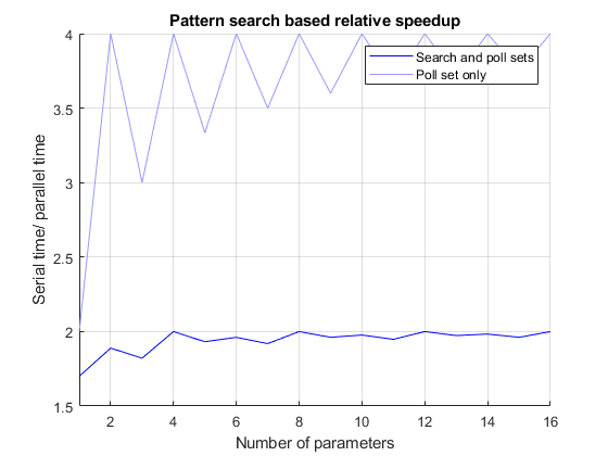
The dark curve is the speedup when the solution and poll sets are evaluated and the lighter lower curve the speedup when only the poll set is evaluated. The expected speedup over an optimization should lie between the two curves. Notice that even with only one parameter, a pattern search method benefits from distribution. Also recall that for the HL20 aircraft problem, which has 3 parameters, the quad core speedup observed was 2.81 which matches well with this plot.
Overhead of Distributing an Optimization
In the previous sections, the overhead associated with performing the optimization in parallel was ignored. Including this overhead gives an indication of the complexity of a simulation that will benefit from distributed optimization.
The overhead associated with running an optimization in parallel primarily results from two sources:
opening the parallel pool
loading the Simulink model and performing an update diagram on the model
There is also some overhead associated with transferring data to and from the remote processors. Simulink Design Optimization relies on shared paths to provide remote processors access to models and the returned data is limited to objective and constraint violation values. Therefore, this overhead is typically much smaller than opening the MATLAB® pool and loading the model. This was true for the HL20 aircraft optimization but may not be true in all cases. However, the analysis shown below can be extended to cover additional overhead.
findOverhead = false; % Set true to compute overhead for your system.
if findOverhead
  % Compute overhead.
  wState = warning('off','MATLAB:dispatcher:pathWarning');
  t0 = datetime('now');           %Current time
  parpool                         %Open the parallel pool
  load_system('airframe_demo')    %Open a model
  set_param('airframe_demo','SimulationCommand','update')  %Run an update diagram for the model
  Toverhead = datetime('now')-t0; %Time elapsed
  Toverhead = seconds(Toverhead)  %Convert to seconds
  close_system('airframe_demo')
  delete(gcp)                     %Close the parallel pool
  warning(wState);
else
  % Use overhead observed from experiments.
  Toverhead = 28.6418;
end
Let us consider a gradient-based algorithm with the following number of serial simulations per iteration:
Nw  = 4;                      %Four parallel processors
Np  = 4;                      %Four parameters optimized
Nls = 2;                      %Assume 2 line search simulations
Nss = 1+Np*2+Nls;             %Serial simulations without parallel computing
Nps = 1+ceil(Np/Nw)*2+Nls;    %Serial simulations with parallel computing
The speedup is now computed as the ratio of the total parallel time including overhead to the total serial time. For worst case analysis, assume the optimization terminates after one iteration which gives:
Niter = 1;
Ts    = 10:10:60;                %Time to simulate model once
Tst   = Niter*Nss*Ts;            %Total serial optimization time
Tpt   = Niter*Nps*Ts+Toverhead;  %Total parallel optimization time
figure;
hAx  = gca;
xlim([min(Ts) max(Ts)]);
Rp = (Tst)./( Tpt );
line('parent',hAx,'xdata',Ts,'ydata',Rp,'color',[0 0 1]);
Niter = 2^1:4;
for ct = 1:numel(Niter)
   Rp = ( Niter(ct)*Nss*Ts )./(Niter(ct)*Nps*Ts+Toverhead);
   line('parent',hAx,'xdata',Ts,'ydata',Rp,'color',[0.6 0.6 1]);
end
grid on
title('Effect of parallel overhead on optimization speedup')
xlabel('Time to simulate model once')
ylabel('Serial time/ parallel time')
annotation('arrow',[0.55 0.55],[0.45 0.85]);
text(38,2.05,'Increasing number of iterations')
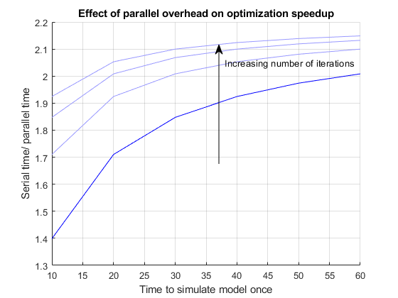
The dark lower curve shows the speedup assuming one iteration while the lighter upper curves indicate speedup with up to 16 iterations.
A similar analysis could be performed for pattern search based optimization. Experience has shown that optimization of complex simulations that take more than 40 seconds to run typically benefit from parallel optimization.
Uncertain Parameters and Their Effect on Parallel Optimization
When using Simulink Design Optimization, you can vary some parameters (say a spring stiffness) and optimize parameters in the face of these variations. The uncertain parameters define additional simulations that need to be evaluated at each iteration. However, conceptually you can think of these additional simulations as extending the simulation without uncertain parameters. This implies that wherever one simulation was carried out, now multiple simulations are carried out. As a result, uncertain parameters do not affect the overhead free optimization speedup and the calculations in earlier sections are valid.
In the case where we considered overhead, uncertain parameters have the effect of increasing the simulation time and reduce the effect of the overhead associated with creating a parallel optimization. To see this consider the following
Nu = [0 10];                        %Number of uncertain scenarios
Nss = (1+Nu)*(1+Np*2+Nls);          %Serial simulations without parallel computing
Nps = (1+Nu)*(1+ceil(Np/Nw)*2+Nls); %Serial simulations with parallel computing
figure;
hAx  = gca;
xlim([min(Ts) max(Ts)]);
for ct = 1:numel(Nu)
   Rp = (Ts*Nss(ct))./(Ts*Nps(ct)+Toverhead);
   line('parent',hAx,'xdata',Ts,'ydata',Rp,'color',[0 0 1]);
end
grid on
title('Effect of uncertain parameters on optimization speedup')
xlabel('Time to simulate model once')
ylabel('Serial time/ parallel time')
annotation('arrow',[0.45 0.45],[0.4 0.9])
text(31,2.05,'Increasing number of uncertain variables')
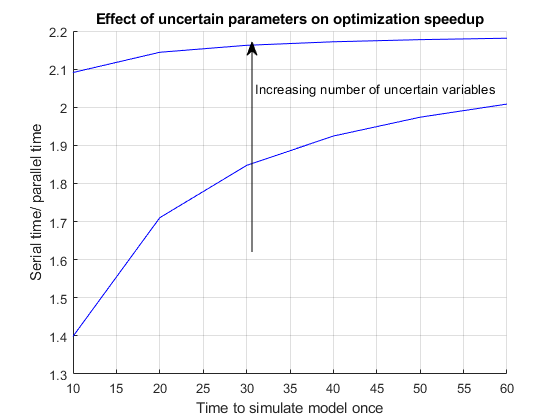
The bottom curve is the case with no uncertain parameters while the top curve is the case with an uncertain parameter that can take on 10 distinct values.
You can also select a web site from the following list:
Americas
- América Latina (Español)
- Canada (English)
- United States (English)
Europe
- Belgium (English)
- Denmark (English)
- Deutschland (Deutsch)
- España (Español)
- Finland (English)
- France (Français)
- Ireland (English)
- Italia (Italiano)
- Luxembourg (English)
- Netherlands (English)
- Norway (English)
- Österreich (Deutsch)
- Portugal (English)
- Sweden (English)
- Switzerland
- United Kingdom (English)