Plot Route and Speed on a Map Using MAT-File Logging on an Android Device

This example uses:

This example shows you how to plot the route and speed of your journey on a web map using MAT-file logging on an Android® device. GPS coordinates are collected in MAT-files and used to plot the route and speed.

Introduction

Simulink® Support Package for Android Devices supports logging of signals from your Simulink model on an Android device in the MAT-file format. MAT-file logging enables you to monitor the behavior of the signal and perform analysis of historical data.

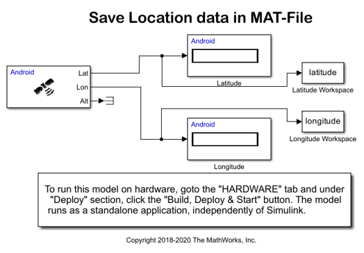
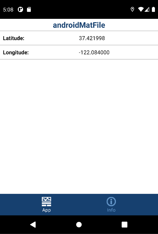
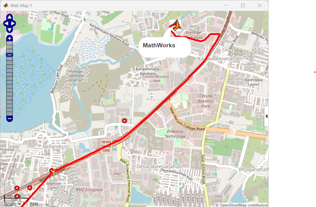
To demonstrate MAT-file logging on Android devices, this example uses a androidMatFile Simulink model. This model logs GPS (latitude and longitude) coordinates on your Android device in multiple MAT-files. You can then import the MAT-files into your computer and use the files for further analysis in MATLAB®. In this example, the MAT-files are used to plot the route and speed of your journey on a web map. The polyline on the map represents the route. The color of the polyline represents the speed.

Prerequisite

Before you start with this example, we recommend you to read:

Getting Started with Android Devices example
Log Signals in MAT-Files on an Android Device documentation

Required Hardware

Android device
USB cable

Step 1: Configure Simulink Model

Note: Before you proceed with this step, you must install the Simulink Support Package for Android Devices as described in Install Support for Android Devices.

1. Open the androidMatFile Simulink model.

2. On the Modeling tab of the toolstrip, select Model Settings.

3. In the Configuration Parameters dialog box, select Hardware Implementation. Verify that the Hardware board parameter is set to Android Device.

4. From the Groups list under Target hardware resources, select Device options.

5. From the Device list, select your Android device. If your device is not listed, click Refresh.

Note: If your device is not listed even after clicking Refresh, ensure that you have enabled the USB debugging option on your device. To enable USB debugging, enter androidhwsetup in the MATLAB Command Window and follow the onscreen instructions.

Step 2: Enable MAT-file Logging

1. In the Configuration Parameters dialog box, browse to Code Generation > Interface > Advanced Parameters and verify these settings:

a. The MAT-file logging option is selected.

b. The MAT-file variable name modifier list is set as rt_. Using this list, you can specify if rt_ is to be added as a prefix or a suffix to the variable name in the MAT-file. To use a variable name without any modification, select none.

2. Click Apply to save the changes and then click OK.

Step 3: Configure To Workspace Blocks

1. In the Simulink model, double-click the To Workspace blocks, Latitude Workspace and Longitude Workspace. Verify these parameter values:

    Parameter                 | Value                                         | Description
  _ _ _ _ _ _ _ _ _ _ _ _ _ _ _ _ _ _ _ _ _ _ _ _ _ _ _ _ _ _ _ _ _ _ _ _ _ _ _ _ _ _ _ _ _ _ _ _ _ _ _ _ _ _ _ _ _ _ _ _ _ _ _ _ _ _ _ _ _ _ _ _
    Variable name             | latitude (in the Latitude Workspace block)    | The variable name by which the latitude and longitude
                              | longitude (in the Longitude Workspace block)  | coordinates are to be logged in the MAT-file.
    Limit data points to last | 500                                           | The number of coordinates to be logged in the MAT-file.
    Save format               | Structure With Time                           | Save data as a structure with associated time information.

2. Click Apply to save the changes and then click OK.

Step 4: Specify Simulation Time and Deploy Simulink Model on Android Device

Note: Before you proceed with this step,

You must have a Simulink Coder™ license.
Ensure that the Location Settings of your Android device is turned on.

1. On the Simulink model toolbar, the Simulation stop time parameter specifies the duration for which the coordinates are logged in the MAT-files. For example, if the Simulation stop time parameter is 10.0 seconds, the coordinates are logged for 10.0 seconds, and then the logging stops. However, the model continues to run for an indefinite time. In this example, Simulation stop time is specified as inf, indicating that the coordinates will be logged indefinitely.

2. On the Hardware tab of the Simulink model, in the Mode section, select Run on board and then click Build, Deploy & Start. This action builds and downloads the model on your Android device. After a successful deployment, the application starts running on the device and logs the latitude and longitude coordinates in MAT-files.

3. Walk while holding the device. Make sure that you walk at least for the duration specified by the Simulation stop time parameter.

Step 5: Import MAT-files from Android Device

1. Copy the MAT-files from the Android device into MATLAB by entering this command in the MATLAB Command Window:

   [<variable1>, <variable2>] = codertarget.android.internal.getFiles('<modelname>')

variable1 is a MATLAB variable that displays the status of the copy operation. variable2 displays the list of the MAT-files copied to MATLAB. In an unsuccessful copy operation, variable2 displays the error message.

For example,

   [result, matFiles] = codertarget.android.internal.getFiles('androidMatFile')

   result =

   matFiles =

       'Successfully pulled following files from device:
        androidMatFile_1_1.mat
        androidMatFile_1_2.mat
        androidMatFile_1_3.mat
        androidMatFile_1_4.mat
        androidMatFile_1_5.mat
        androidMatFile_1_6.mat
        androidMatFile_1_7.mat
        androidMatFile_1_8.mat
      '

After successfully copying the files, the value of the result variable becomes 0. The matFiles variable displays the names of the MAT-files copied to MATLAB. You can also see the copied files in the MATLAB Current Folder window.

If MATLAB encounters any issue when copying the files, the value of the result variable changes to a nonzero value. The matFiles variable displays the corresponding error message.

2. Combine all the MAT-files into a single MAT-file by using the Android_MAT_stitcher command. This command combines all the MAT-files starting with the same name in the current directory into a single file. The order of the stitching is based on the numeric characters found at the end of the file name. The name of the stitched file ends with __stitched.mat.

Note: A preloaded stitched file is available for you to use. To use the preloaded file, directly load the file as described in the next step of this section.

   Android_MAT_stitcher(dir('*.mat'));

For information on the stitcher command, enter edit('Android_MAT_stitcher.m');.

3. Load the stitched MAT-file.

   load('<stitchedMATfile>');

For example,

   load('androidMatFile_1__stitched.mat');

4. To view the logged latitude and longitude coordinates, double-click the rt_simout and rt_simout1 variables in the Workspace window, respectively.

Step 6: Calculate the Speed Using Latitude and Longitude

1. Assign the coordinate values to the MATLAB variables.

   lat = rt_simout.signals.values;
   lon = rt_simout1.signals.values;

2. Calculate the speed of your journey.

   l = length(lat);
   radius= 6371.00;
   time =1;
   spd =zeros(l,1);
   for t= 1:l
       if t>1
           oldLat = lat(t);
           oldlon = lon(t);
           newLat = lat(t-1);
           newLon = lon(t-1);
           dLat = deg2rad(newLat-oldLat);
           dLon = deg2rad(newLon- oldlon);
           a = sin(dLat/2) * sin(dLat/2) +  ...
               cos(deg2rad(oldLat)) *cos(deg2rad(newLat)) * ...
               sin(dLon/2) * sin(dLon/2);
           c = 2 * asin(sqrt(a));
           spd(t) =  (6371.00 * c*1609.00 *60)/1000;
       else
           spd(t) = 0;
       end
   end

Step 7: Associate Speed Range with Color Values

To represent the speeds with discrete colors, bin the speed values.

   nBins = 10;
   binSpacing = (max(spd) - min(spd))/nBins;
   binRanges = min(spd):binSpacing:max(spd)-binSpacing;

   % To enclose the values above the last bin, add an inf to binRanges.
   binRanges(end+1) = inf;

   %|histc| determines the bin for each speed value.
   [~, spdBins] = histc(spd, binRanges);

Step 8: Split Latitude and Longitude Data by Speed

Note: Before you proceed with this step, you must have a Mapping Toolbox™ license.

MATLAB creates discontinuous line segments for every speed bin. Each of these segments are assigned the same color. This creates far fewer total line segments than treating every adjacent pair of latitude and longitude values as their own line segments.

Obtain the geographic vector features of these segments using the geoshape command from the Mapping Toolbox.

   spdBins = spdBins';

  %Create an empty geoshape vector
   s = geoshape();

   for k = 1:nBins

       % Store only the lat and lon values that match the current bin. Specify the
       % non-matching values as NaN. NaN is interpreted as breaks in the line segments.
       latValid = nan(1, length(lat));
       latValid(spdBins==k) = lat(spdBins==k);

       lonValid = nan(1, length(lon));
       lonValid(spdBins==k) = lon(spdBins==k);

       % For a continuous path, store the lat and lon values that occur after
       % transitioning from the current speed bin to the next speed bin.
       transitions = [diff(spdBins) 0];
       insertionInd = find(spdBins==k & transitions~=0) + 1;

       % Preallocate space and insert extra lat and lon values.
       latSeg = zeros(1, length(latValid) + length(insertionInd));
       latSeg(insertionInd + (0:length(insertionInd)-1)) = lat(insertionInd);
       latSeg(~latSeg) = latValid;

       lonSeg = zeros(1, length(lonValid) + length(insertionInd));
       lonSeg(insertionInd + (0:length(insertionInd)-1)) = lon(insertionInd);
       lonSeg(~lonSeg) = lonValid;

       % Assign the lat and lon values to the geoshape vector.
       s(k) = geoshape(latSeg, lonSeg);

end

Step 9: Create Web Map and Route Overlay

1. Open a web map.

   wm = webmap('Open Street Map');

2. On the map, plot your current location for a reference. In this example, the MathWorks® Bangalore, India, office is marked.

   mwLat = 12.9434;
   mwLon = 77.6914;
   name = 'MathWorks';
   iconDir = fullfile(matlabroot,'toolbox','matlab','icons');
   iconFilename = fullfile(iconDir, 'matlabicon.gif');
   wmmarker(mwLat, mwLon, 'FeatureName', name, 'Icon', iconFilename);

3. Represent each speed bin with different colors using the autumn command. The command creates an nBins-by-3 array. Each row in the array contains the red, green, and blue intensities for the color representing each bin.

   colors = autumn(nBins);

4. Draw a line overlay on the web map using the wmline command. The map provides a visual representation of the route and the speed of your journey. The polyline represents the route. The color of the polyline represents the speed of your journey.

   wmline(s, 'Color', colors, 'Width', 5);

5. To control the zoom level of the web map, use the wmzoom command.

   wmzoom(16);