Automotive Suspension
This example shows how to model a simplified half-car system that includes independent front and rear vertical suspensions. The model also incorporates body pitch and bounce degrees of freedom. The example provides a description of the model to demonstrate how simulation can be used to investigate ride characteristics. You can use this model in conjunction with a powertrain simulation to study longitudinal shuffle resulting from changes in throttle setting.
Analysis and Physics
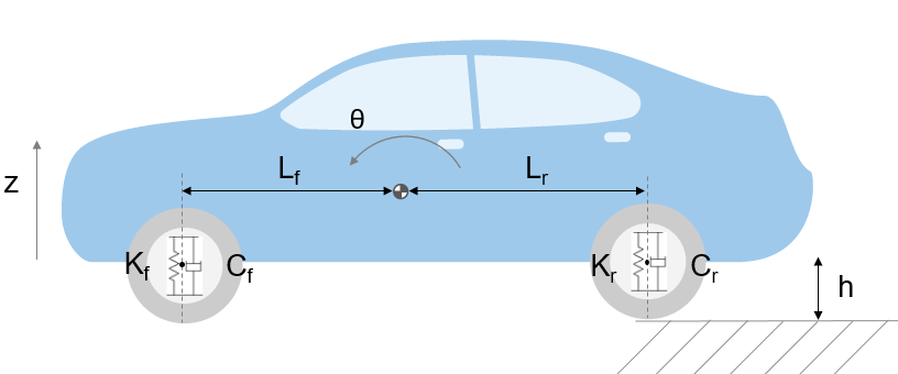
The illustration shows the modeled characteristics of the half-car. The front and rear suspensions are modeled as spring/damper systems. A more detailed model would include a tire model and damper nonlinearities, such as velocity-dependent damping (with greater damping during rebound than compression). The vehicle body has pitch and bounce degrees of freedom, which are represented in the model by four states: vertical displacement, vertical velocity, pitch angular displacement, and pitch angular velocity. A full model with six degrees of freedom can be implemented using vector algebra blocks to perform axis transformations and force, displacement, and velocity calculations.
Equation 1 describes the influence of the front suspension on the bounce (i.e. vertical degree of freedom):

where:


Equations 2 describe pitch moments due to the suspension.


where:

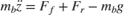
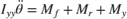
Equations 3 resolves the forces and moments result in body motion, according to Newton's Second Law:
where:


Model
Open the model.
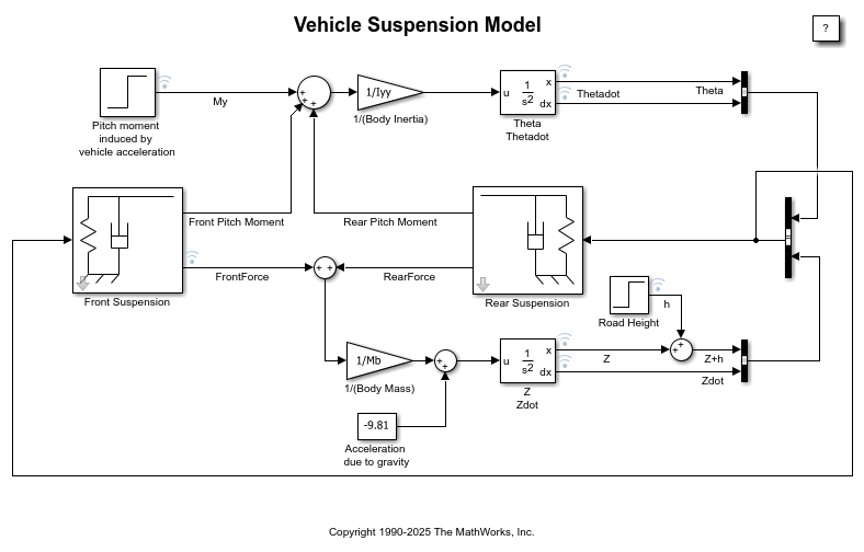
The suspension model has two inputs, and both input blocks are blue on the model diagram. The first input is the road height. A step input here corresponds to the vehicle driving over a road surface with a step change in height. The second input is a horizontal force acting through the center of the wheels, resulting from braking or acceleration maneuvers. This input appears only as a moment about the pitch axis because longitudinal body motion is not modeled.
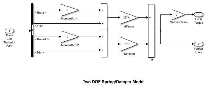
The spring/damper subsystem that models the front and rear suspensions is shown above. Right-click the Front Suspension or Rear Suspension block. Select Edit Mask > Look Under Mask to see the front or rear suspension subsystem. The suspension subsystems model Equations 1-3. The Simulink® diagram uses the Gain and Summation blocks to implement Equations 1-3.
The differences between the front and rear are accounted for as follows. Because the subsystem is a masked block, a different data set (L, K and C) can be entered for each instance. Furthermore, L is thought of as the Cartesian coordinate x, being negative or positive with respect to the origin, or center of gravity. Thus, Kf, Cf, and -Lf are used for the front suspension block whereas Kr, Cr, and Lr are used for the rear suspension block.
Run Simulation
To run this model, on the Simulation tab, click Run. Initial conditions are loaded into the model workspace from the sldemo_suspdat.m file. To see the contents of the model workspace, in the Simulink Editor, on the Modeling tab, under Design, select Model Explorer. In the Model Explorer, look under the contents of the sldemo_suspn model and select "Model Workspace". Loading initial conditions in the model workspace prevents any accidental modifications of parameters and keeps MATLAB workspace clean.
The model logs relevant data to MATLAB workspace in a data structure called sldemo_suspn_output. Type the name of the structure to see what data it contains.
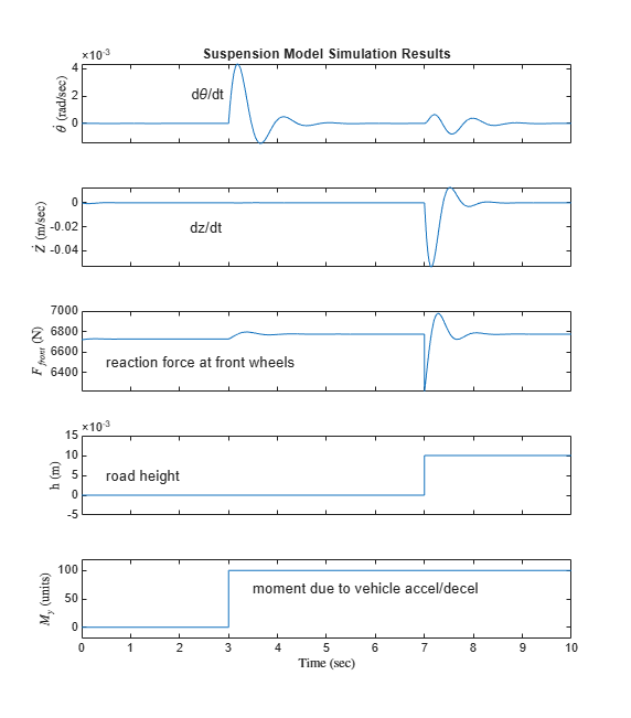
Simulation results are displayed above. The results are plotted by the sldemo_suspgraph.m file. The default initial conditions are given in Table 1.
Table 1: Default initial conditions
Lf = 0.9;    % front hub displacement from body gravity center (m)
Lr = 1.2;    % rear hub displacement from body gravity center (m)
Mb = 1200;   % body mass (kg)
Iyy = 2100;  % body moment of inertia about y-axis (kg m^2)
kf = 28000;  % front suspension stiffness (N/m)
kr = 21000;  % rear suspension stiffness (N/m)
cf = 2500;   % front suspension damping (N sec/m)
cr = 2000;   % rear suspension damping (N sec/m)
This model allows you to simulate the effects of changing the suspension damping and stiffness, thereby investigating the tradeoff between comfort and performance. In general, racing cars have very stiff springs with a high damping factor, whereas passenger vehicles have softer springs and a more oscillatory response.