Understanding Model Architecture
When evaluating the modeling guidelines for your project, it is important that you understand the architecture of your controller model, such the function/subfunction layers, schedule layer, control flow layer, section layer, and data flow layer.
Hierarchical Structure of a Controller Model
This section provides a high-level overview of the hierarchical structuring in a basic model, using a controller model as an example. This table defines the layer concepts in a hierarchy.
| Layer concept | Layer purpose | |
Top Layer | Function layer | Broad functional division |
| Schedule layer | Expression of execution timing (sampling, order) | |
Bottom Layer | Sub function layer | Detailed function division |
| Control flow layer | Division according to processing order (input → judgment → output, etc.) | |
| Selection layer | Division (select output with Merge) into a format that switches and activates the active subsystem | |
| Data flow layer | Layer that performs one calculation that cannot be divided |
When applying layer concepts:
Layer concepts shall be assigned to layers and subsystems shall be divided accordingly.
When a layer concept is not needed, it does not need to be allocated to a layer.
Multiple layer concepts can be allocated to one layer.
When building hierarchies, division into subsystems for the purpose of saving space within the layer shall be avoided.
Top Layer
Layout methods for the top layer include:
Simple control model — Represents both the function layer and schedule layer in the same layer. Here, function is execution unit. For example, a control model has only one sampling cycle and all functions are arranged in execution order.
Complex control model Type α — The schedule layer is positioned at the top. This method makes integration with the code easy, but functions are divided, and the readability of the model is impaired.
Complex control model Type β — Function layers are arranged at the top and schedule layers are positioned below the individual function layers.

Function Layers and Sub-Function Layers
When modeling function and sub-function layers:
Subsystems shall be divided by function, with the respective subsystems representing one function.
One function is not always an execution unit so, for that reason, the respective subsystem is not necessarily an atomic subsystem. In the type β example below, it is more appropriate for a function layer subsystem to be a virtual subsystem. Algebraic loops are created when these change into atomic subsystems.
Individual functional units shall be described.
When the model includes multiple large functions, consider using model references for each function to partition the model.

Schedule Layers
When scheduling layers:
System sampling intervals and execution priority shall be set. Use caution when setting multiple sampling intervals. In connected systems with varying sampling intervals, ensure that the system is split for each sampling interval. This minimizes the RAM needed to store previous values in the situation where the processing of signals values differs for fast cycles and slow cycles.
Priority ranking shall be set. This is important when designing multiple, independent functions. When possible, computation sequence for all subsystems should be based on subsystem connections.
Two different types of priority rankings shall be set, one for different sampling intervals and the other for identical sampling rates.
There are two types of methods that can be used for setting sampling intervals and priority rankings:
For subsystems and blocks, set the block parameter sample time and block properties priority.
When using conditional subsystems, set independent priority rankings to match the scheduler.
Patterns exist for many different conditions, such as the configuration parameters for custom sampling intervals, atomic subsystem settings, and the use of model references. The use of a specific pattern is closely linked to the code implementation method and varies significantly depending on the status of the project. Models that are typically affected include:
Models that have multiple sampling intervals
Models that have multiple independent functions
Usage of model references
Number of models (and whether there is more than one set of generated code)
For the generated code, affected factors include:
Applicability of a real-time operating system
Consistency of usable sampling intervals and computation cycles to be implemented
Applicable area (application domain or basic software)
Source code type: AUTOSAR compliant - not compliant - not supported.
Control Flow Layers
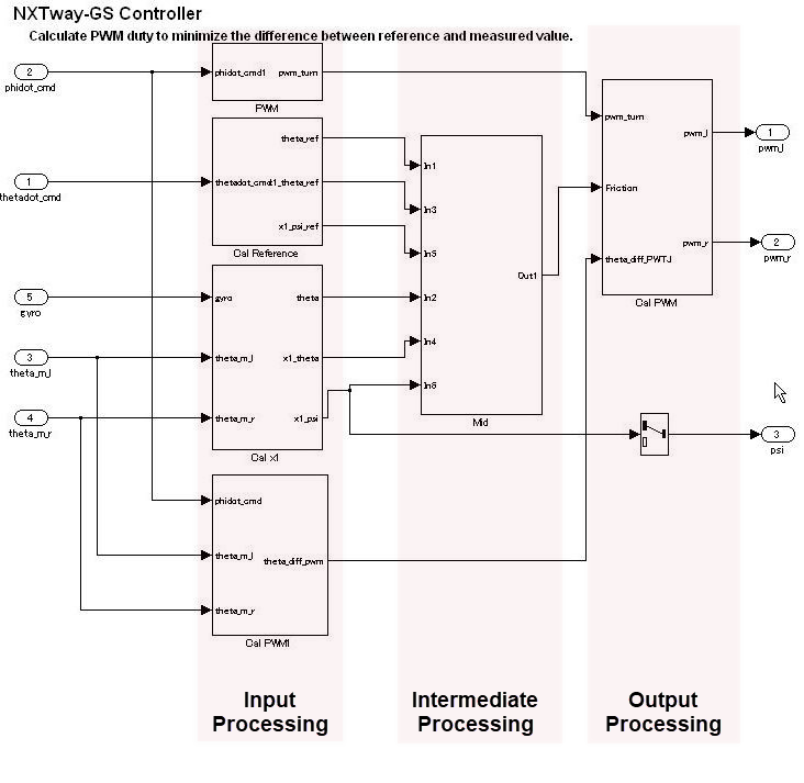
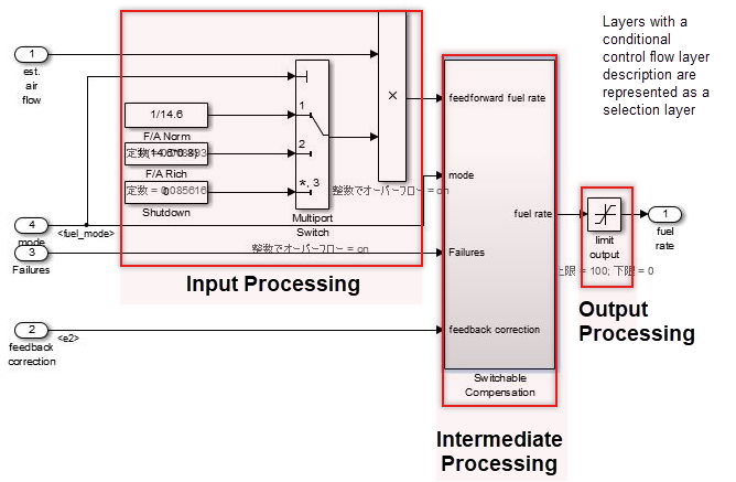
In the hierarchy, the control layer expresses all input processing, intermediate processing, and output processing by using one function. The arrangement of blocks and subsystems is important in this layer. Multiple, mixed small functions should be grouped by dividing them between the three largest stages of input processing, intermediate processing and output processing, which forms the conceptual basis of control. The general configuration occurs close to the data flow layer and is represented in the horizontal line. The difference in a data flow layer is its construction from multiple subsystems and blocks.
In control flow layers, the horizontal direction indicates processing with different significance; blocks with the same significance are arranged vertically.
Block groups are arranged horizontally and are given a provisional meaning. Red borders, which signify the delimiter for processing that is not visible, correspond to objects called virtual objects. Using annotations to mark the delimiters makes it easier to understand.
Control flow layers can co-exist with blocks that have a function. They are positioned between the sub-function layer and the data flow layer. Control flow layers are used when:
The number of blocks becomes too large
All is described in the data flow layer
Units that can be given a minimum partial meaning are made into subsystems
Placement in the hierarchy organizes the internal layer configuration and makes it easier to understand. It also improves maintainability by avoiding the creation of unnecessary layers.
When the model consists solely of blocks and does not include a mix of subsystems, if the horizontal layout can be split into input/intermediate/output processing, it is considered a control flow layer.
Selection Layers
When modeling selection layers:
Selection layers should be written vertically or side-by-side. There is no significance to which orientation is chosen.
Selection layers shall mix with control flow layers.
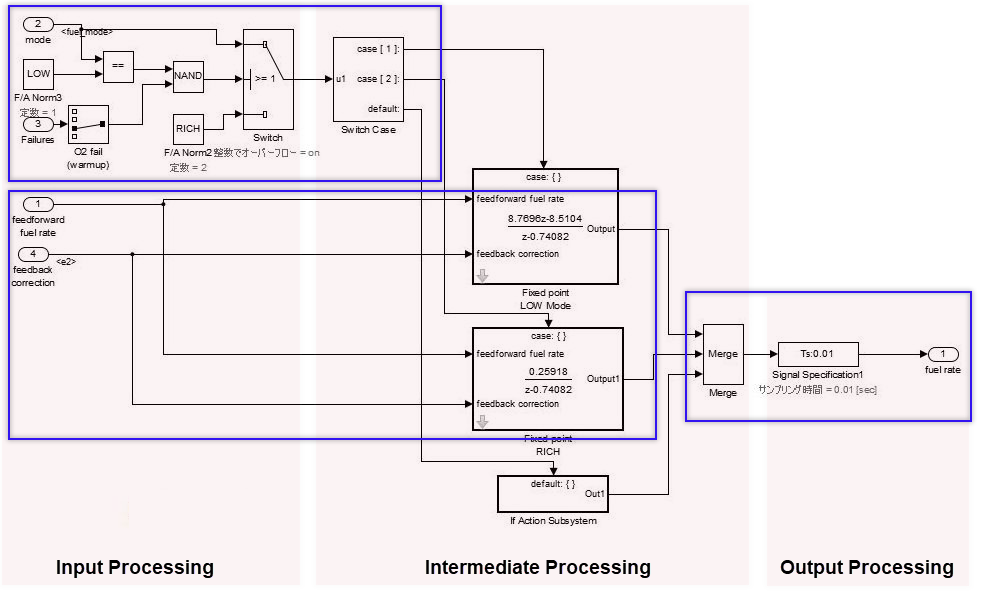
When a subsystem has switch functions that allow only one subsystem to run depending on the conditional control flow inside the red border, it is referred to as a selection layer. It is also described as a control flow layer because it structures input processing/intermediate processing (conditional control flow)/output processing.
In the control flow layer, the horizontal direction indicates processing with different significance. Parallel processing with the same significance is structured vertically. In selection layers, no significance is attached to the horizontal or vertical direction, but they show layers where only one subsystem can run. For example:
Switching coupled functions to run upwards or downwards, changing chronological order
Switching the setting where the computation type switches after the first time (immediately after reset) and the second time
Switching between destination A and destination B
Data Flow Layers
A data flow layer is the layer below the control flow layer and selection layer.
A data flow layer represents one function as a whole; input processing, intermediate processing and output processing are not divided. For instance, systems that perform one continuous computation that cannot be split.
Data flow layers cannot coexist with subsystems apart from those where exclusion conditions apply. Exclusion conditions include:
Subsystems where reusable functions are set
Masked subsystems that are registered in the Simulink® standard library
Masked subsystems that are registered in a library by the user
Example of a simple data flow layer.
Example of a complex data flow layer.
When input processing and intermediate processing cannot be clearly divided as described above, they are represented as a data flow layer.
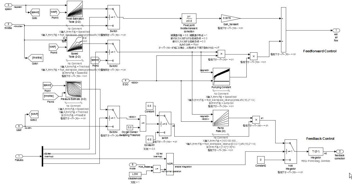
A data flow layer becomes complicated when both the feed forward reply and feedback reply from the same signal are computed at the same time. Even when the number of blocks in this type of cases is large, the creation of a subsystem should not be included in the design when the functions cannot be clearly divided. When meaning is attached through division, it should be designed as a control flow layer.
Relationship Between Simulink Models and Embedded Implementation
Running an actual micro controller requires embedding the code that is generated from the Simulink model into the micro controller. This requirement affects the configuration Simulink model and is dependent on:
The extent to which the Simulink model will model the functions
How the generated code is embedded
The schedule settings on the embedded micro controller
The configuration is affected significantly when the tasks of the embedded micro controller differs from those modeled by Simulink.
Scheduler Settings in Embedded Software
The scheduler in embedded software has single-task and multi-task settings.
Single-task schedule settings
A single-task scheduler performs all processing by using basic sampling. Therefore, when processing of longer sampling is needed, the function is split so the CPU load is as evenly distributed as possible, and then processed using basic sampling. However, as equal splitting is not always possible, functions may not be able to be allocated to all cycles.
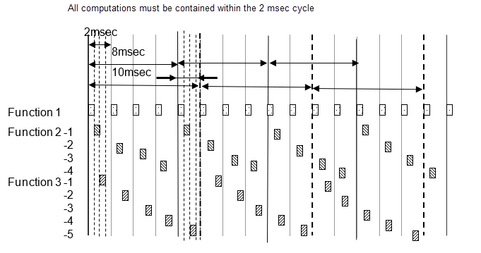
For example, basic sampling is 2 millisecond, and sampling rates of 2 millisecond, 8 millisecond and 10 millisecond exist within the model. An 8 millisecond function is executed once for every four 2 millisecond cycles, and a 10 millisecond function is executed once for every five. The number of executions is counted every 2 millisecond and the sampling function specified by this frequency is executed. Attention needs to be paid to the fact that the 2 millisecond, 8 millisecond and 10 millisecond cycles are all computed with the same 2 millisecond. Because all computations need to be completed within 2 millisecond, the 8 millisecond and 10 millisecond functions are split into several and adjusted so that all 2 millisecond computations are of an almost equal volume.
The following diagram shows the 8 millisecond function split into 4 and the 10 millisecond function split into 5.
| Functions | Fundamental frequency | Offset |
| 8millisecond | 0millisecond | |
| 2-2 | 8millisecond | 2millisecond |
| 2-3 | 8millisecond | 4millisecond |
| 2-4 | 8millisecond | 6millisecond |
| 3-1 | 10millisecond | 0millisecond |
| 3-2 | 10millisecond | 2millisecond |
| 3-3 | 10millisecond | 4millisecond |
| 3-4 | 10millisecond | 6millisecond |
| 3-5 | 10millisecond | 8millisecond |
To set frequency-divided tasking:
Clear configuration parameter Treat each discrete rate as a separate task.
For the Atomic Subsystem block parameter Sample time, enter the sampling period offset values. A subsystem for which a sampling period can be specified is referred to as an atomic subsystem.

Multi-task scheduler settings
Multi-task sampling is executed by using a real-time OS that supports multi-task sampling. In single-task sampling, equalizing the CPU load is not done automatically, but a person divides the functions and allocates them to the appointed task. In multi-task sampling, the CPU performs the computations automatically in line with the current status; there is no need to set detailed settings. Computations are performed and results are output starting from the task with the highest priority, but the task priorities are user-specified. Typically, fast tasks are assigned highest priority. The execution order for this task is user-specified.

It is important that computations are completed within the cycle, including slow tasks. When the processing of a high priority computation finishes and the CPU is available, the computation for the system with the next priority ranking begins. A high priority computation process can interrupt a low priority computation, which is then aborted so the high priority computation process can execute first.
Effect of Connecting Subsystems with Sampling Differences
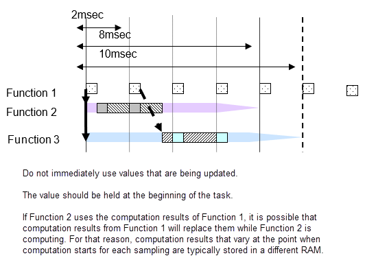
If subsystem B with a 20 millisecond sampling interval uses the output of subsystem A with a 10 millisecond sampling interval, the output result of subsystem A can change while subsystem B is computing. If the values change partway through, the results of subsystem B’s computation may not be as expected. For example, a comparison is made in subsystem B’s first computation with the subsystem A output, and the result is computed with the conditional judgment based on this output. At this point, the comparison result is true. It is then compared again at the end of subsystem B; if the output from A is different, then the result of the comparison can be false. Generally, in this type of function development it may happen that the logic created with true, true has become true, false, and an unexpected computation result is generated. To avoid this type of malfunction, when there is a change in task, output results from subsystem A are fixed immediately before they are used by subsystem B as they are used in a different RAM from that used by the subsystem A output signals. In other words, even if subsystem A values change during the process, the values that subsystem B are looking at is in a different RAM, so no effect is apparent.
When a model is created in Simulink and a subsystem is connected that has a different sampling interval in Simulink, Simulink automatically reserves the required RAM.
However, if input values are obtained with a different sampling interval through integration with hand-coded code, the engineer who does the embedding work should design these settings. For example, in the RTW concept using AUTOSAR, different RAMs are all defined at the receiving and exporting side.
Single-task scheduler settings
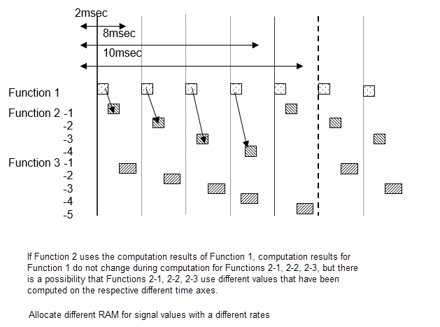
Signal values are the same within the same 2 millisecond cycle, but when there are different 2 millisecond cycles, the computation value differs from the preceding one. When Function 2-1 and 2-2 uses signal A of Function 1, be aware that 2-1 and 2-2 uses results from different times.
Multi-task scheduler settings
For multi-task, you cannot specify at what point to use the computation result to use. With multi-task, always store signals for different tasks in new RAM.
Before new computations are performed within the task, all values are copied.