Estimate State for Digital Clock
This example shows how to estimate the high and low state levels for digital clock data. In contrast to analog voltage signals, signals in digital circuits have only two states: HIGH and LOW. Information is conveyed by the pattern of high and low state levels.
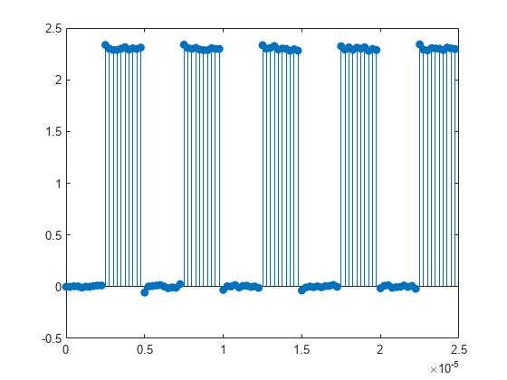
Load clockex.mat into the MATLAB® workspace. clockex.mat contains a 2.3 volt digital clock waveform sampled at 4 megahertz. Load the clock data into the variable x and the vector of sampling times in the variable t. Plot the data.
load('clockex.mat','x','t')
stem(t,x,'filled')
Determine the high and low state levels for the clock data using statelevels.
levels = statelevels(x)
levels = 1×2

    0.0027    2.3068
This is the expected result for the 2.3 volt clock data, where the noise-free low-state level is 0 volts and the noise-free high-state level is 2.3 volts.
Use the estimated state levels to convert the voltages into a sequence of zeros and ones. The sequence of zeros and ones is a binary waveform representation of the two states. To make the assignment, use the following decision rule:
Assign any voltage within a 3%-tolerance region of the low-state level the value 0.
Assign any voltage within a 3%-tolerance region of the high-state level the value 1.
Determine the widths of the 3%-tolerance regions around the low- and high-state levels.
tolwd = 3/100*diff(levels);
Use logical indexing to determine the voltages within a 3%-tolerance region of the low-state level and the voltages within a 3%-tolerance region of the high-state level. Assign the value 0 to the voltages within the tolerance region of the low-state level and 1 to the voltages within the tolerance region of the high-state level. Plot the result.
y = zeros(size(x));
y(abs(x-min(levels))<=tolwd) = 0;
y(abs(x-max(levels))<=tolwd) = 1;

subplot(2,1,1)
stem(t,x,'filled')
ylabel('Volts')
subplot(2,1,2)
stem(t,y,'filled')
ylabel('\{0,1\}')
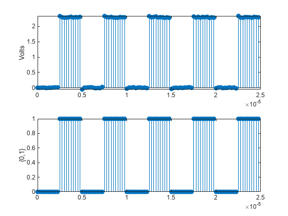
The decision rule has assigned all the voltages to the correct state.