Detect a Distorted Signal in Noise
The presence of noise often makes it difficult to determine the spectral content of a signal. Frequency analysis can help in such cases.
Consider for example the simulated output of a nonlinear amplifier that introduces third-order distortion.
The input signal is a 180 Hz unit-amplitude sinusoid sampled at 3.6 kHz. Generate 10000 samples.
N = 1e4;
n = 0:N-1;
fs = 3600;
f0 = 180;
t = n/fs;
y = sin(2*pi*f0*t);
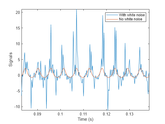
Add unit-variance white noise to the input. Model the amplifier using a third-order polynomial. Pass the input signal through the amplifier using polyval. Plot a section of the output. For comparison plot the output of a pure sinusoid.
rng default
noise = randn(size(y));

dispol = [0.5 0.75 1 0];
out = polyval(dispol,y+noise);

ns = 300:500;

plot(t(ns),[out(ns);polyval(dispol,y(ns))])
xlabel('Time (s)')
ylabel('Signals')
axis tight
legend('With white noise','No white noise')

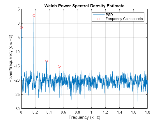
Use pwelch to compute and plot the power spectral density of the output.
[pxx,f] = pwelch(out,[],[],[],fs);

pwelch(out,[],[],[],fs)

Because the amplifier introduces third-order distortion, the output signal is expected to have:
A DC (zero-frequency) component;
A fundamental component with the same frequency as the input, 180 Hz;
Two harmonics -- frequency components at twice and three times the frequency of the input, 360 and 540 Hz.
Verify that the output is as expected for a cubic nonlinearity.
[pks,lox] = findpeaks(pxx,'NPeaks',4,'SortStr','descend');

hold on
plot(f(lox)/1000,10*log10(pks),'or')
hold off

legend('PSD','Frequency Components')

components = sort([f(lox) f0*(0:3)'])'
components = 2×4

    0.8789  180.1758  360.3516  540.5273
         0  180.0000  360.0000  540.0000
pwelch works by dividing the signal into overlapping segments, computing the periodogram of each segment, and averaging. By default, the function uses eight segments with 50% overlap. For 10000 samples, this corresponds to 2222 samples per segment.
Dividing the signal into shorter segments results in more averaging. The periodogram is smoother, but has lower resolution. The higher harmonic cannot be distinguished.
pwelch(out,222,[],[],fs)

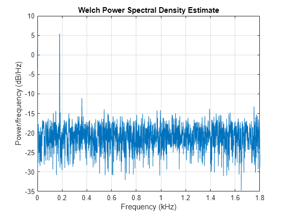
Dividing the signal into longer segments increases the resolution, but also the randomness. The signal and the harmonics are precisely at the expected locations. However, there is at least one spurious high-frequency peak with more power than the higher harmonic.
pwelch(out,4444,[],[],fs)
