Robust Stability, Robust Performance, and Mu Analysis
This example shows how to use Robust Control Toolbox™ to analyze and quantify the robustness of feedback control systems. It also provides insight into the connection with mu analysis and the mussv function.
System Description
Figure 1 shows the block diagram of a closed-loop system. The plant model is uncertain and the plant output must be regulated to remain small in the presence of disturbances and measurement noise .
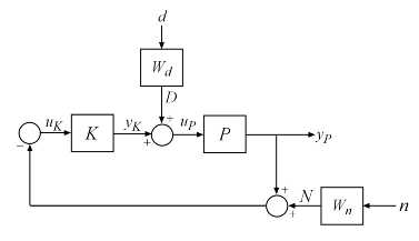
Figure 1: Closed-loop system for robustness analysis
Disturbance rejection and noise insensitivity are quantified by the performance objective
where and are weighting functions reflecting the frequency content of and . Here is large at low frequencies and is large at high frequencies.
Wd = makeweight(100,.4,.15);
Wn = makeweight(0.5,20,100);
bw = bodeplot(Wd,'b--',Wn,'g--');
bw.PhaseVisible = "off";
bw.Title.String = "Performance Weighting Functions";
bw.Responses(1).Name = "Input disturbance";
bw.Responses(2).Name = "Measurement noise";
bw.LegendVisible = "on";

Creating an Uncertain Plant Model
The uncertain plant model P is a lightly-damped, second-order system with parametric uncertainty in the denominator coefficients and significant frequency-dependent unmodeled dynamics beyond 6 rad/s. The mathematical model looks like:
The parameter k is assumed to be about 40% uncertain, with a nominal value of 16. The frequency-dependent uncertainty at the plant input is assumed to be about 30% at low frequency, rising to 100% at 10 rad/s, and larger beyond that. Construct the uncertain plant model P by creating and combining the uncertain elements:
k = ureal('k',16,'Percentage',30);
delta = ultidyn('delta',[1 1],'SampleStateDim',4);
Wu = makeweight(0.3,10,20);
P = tf(16,[1 0.16 k]) * (1+Wu*delta);
Designing a Controller
We use the controller designed in the example "Improving Stability While Preserving Open-Loop Characteristics". The plant model used there happens to be the nominal value of the uncertain plant model created above. For completeness, we repeat the commands used to generate the controller.
K_PI = pid(1,0.8);
K_rolloff = tf(1,[1/20 1]);
Kprop = K_PI*K_rolloff;
[negK,~,Gamma] = ncfsyn(P.NominalValue,-Kprop);
K = -negK;
Closing the Loop
Use connect to build an uncertain model of the closed-loop system of Figure 1. Name the signals coming in and out of each block and let connect do the wiring:
P.u = 'uP';
P.y = 'yP';
K.u = 'uK';
K.y = 'yK';
S1 = sumblk('uP = yK + D');
S2 = sumblk('uK = -yP - N');
Wn.u = 'n';
Wn.y = 'N';
Wd.u = 'd';
Wd.y = 'D';
ClosedLoop = connect(P,K,S1,S2,Wn,Wd,{'d','n'},'yP');
The variable ClosedLoop is an uncertain system with two inputs and one output. It depends on two uncertain elements: a real parameter k and an uncertain linear, time-invariant dynamic element delta.
ClosedLoop
Uncertain continuous-time state-space model with 1 outputs, 2 inputs, 11 states.
The model uncertainty consists of the following blocks:
  delta: Uncertain 1x1 LTI, peak gain = 1, 1 occurrences
  k: Uncertain real, nominal = 16, variability = [-30,30]%, 1 occurrences
Model Properties

Type "ClosedLoop.NominalValue" to see the nominal value and "ClosedLoop.Uncertainty" to interact with the uncertain elements.
Robust Stability Analysis
The classical margins from allmargin indicate good stability robustness to unstructured gain/phase variations within the loop.
allmargin(P.NominalValue*K)
ans = struct with fields:
     GainMargin: [6.2984 10.9082]
    GMFrequency: [1.6108 15.0285]
    PhaseMargin: [79.9815 -99.6214 63.7590]
    PMFrequency: [0.4466 3.1469 5.2304]
    DelayMargin: [3.1254 1.4441 0.2128]
    DMFrequency: [0.4466 3.1469 5.2304]
         Stable: 1
Does the closed-loop system remain stable for all values of k, delta in the ranges specified above? Answering this question requires a more sophisticated analysis using the robstab function.
[stabmarg,wcu] = robstab(ClosedLoop);
stabmarg
stabmarg = struct with fields:
           LowerBound: 1.4668
           UpperBound: 1.4697
    CriticalFrequency: 5.8933
The variable stabmarg gives upper and lower bounds on the robust stability margin, a measure of how much uncertainty on k, delta the feedback loop can tolerate before becoming unstable. For example, a margin of 0.8 indicates that as little as 80% of the specified uncertainty level can lead to instability. Here the margin is about 1.5, which means that the closed loop will remain stable for up to 150% of the specified uncertainty.
The variable wcu contains the combination of k and delta closest to their nominal values that causes instability.
wcu
wcu = struct with fields:
    delta: [1×1 ss]
        k: 23.0548
We can substitute these values into ClosedLoop and verify that these values cause the closed-loop system to be unstable.
format short e
pole(usubs(ClosedLoop,wcu))
ans = 15×1 complex

  -1.2591e+03 + 0.0000e+00i
  -2.0937e+02 + 0.0000e+00i
  -8.2633e+00 + 1.1488e+01i
  -8.2633e+00 - 1.1488e+01i
  -2.4785e+01 + 0.0000e+00i
  -1.9994e+01 + 0.0000e+00i
   2.7123e-13 + 5.8933e+00i
   2.7123e-13 - 5.8933e+00i
  -3.2901e+00 + 0.0000e+00i
  -1.5907e+00 + 2.3468e+00i
  -1.5907e+00 - 2.3468e+00i
  -8.9213e-01 + 0.0000e+00i
  -3.5334e-01 + 0.0000e+00i
  -2.3093e+03 + 0.0000e+00i
  -3.9549e-03 + 0.0000e+00i
Note that the natural frequency of the unstable closed-loop pole is given by stabmarg.CriticalFrequency:
stabmarg.CriticalFrequency
ans =
   5.8933e+00
Connection with Mu Analysis
The structured singular value, or , is the mathematical tool used by robstab to compute the robust stability margin. If you are comfortable with structured singular value analysis, you can use the mussv function directly to compute mu as a function of frequency and reproduce the results above. The function mussv is the underlying engine for all robustness analysis commands.
To use mussv, we first extract the (M,Delta) decomposition of the uncertain closed-loop model ClosedLoop, where Delta is a block-diagonal matrix of (normalized) uncertain elements. The 3rd output argument of lftdata, BlkStruct, describes the block-diagonal structure of Delta and can be used directly by mussv.
[M,Delta,BlkStruct] = lftdata(ClosedLoop);
For robust stability analysis, only the channels of M associated with the uncertainty channels are used. Based on the row/column size of Delta, select the proper columns and rows of M. Remember that the rows of Delta correspond to the columns of M, and vice versa. Consequently, the column dimension of Delta is used to specify the rows of M:
szDelta = size(Delta);
M11 = M(1:szDelta(2),1:szDelta(1));
In its simplest form, mu-analysis is performed on a finite grid of frequencies. Pick a vector of logarithmically-spaced frequency points and evaluate the frequency response of M11 over this frequency grid.
omega = logspace(-1,2,50);
M11_g = frd(M11,omega);
Compute mu(M11) at these frequencies and plot the resulting lower and upper bounds:
mubnds = mussv(M11_g,BlkStruct,'s');

bp = bodeplot(mubnds(1,1),mubnds(1,2));
bp.PhaseVisible = 'off';
bp.MagnitudeUnit = 'abs';
bp.XLimits = [1e-1,1e2];
bp.XLabel.String = "Frequency";
bp.YLabel.String(1) = "Mu upper/lower bounds";
bp.Title.String = "Mu plot of robust stability margins (inverted scale)";

Figure 3: Mu plot of robust stability margins (inverted scale)
The robust stability margin is the reciprocal of the structured singular value. Therefore upper bounds from mussv become lower bounds on the stability margin. Make these conversions and find the destabilizing frequency where the mu upper bound peaks (that is, where the stability margin is smallest):
[pkl,wPeakLow] = getPeakGain(mubnds(1,2));
[pku] = getPeakGain(mubnds(1,1));
SMfromMU.LowerBound = 1/pku;
SMfromMU.UpperBound = 1/pkl;
SMfromMU.CriticalFrequency = wPeakLow;
Compare SMfromMU to the bounds stabmarg computed with robstab. The values are in rough agreement with robstab yielding slightly weaker margins. This is because robstab uses a more sophisticated approach than frequency gridding and can accurately compute the peak value of mu across frequency.
stabmarg
stabmarg = struct with fields:
           LowerBound: 1.4668e+00
           UpperBound: 1.4697e+00
    CriticalFrequency: 5.8933e+00
SMfromMU
SMfromMU = struct with fields:
           LowerBound: 1.4735e+00
           UpperBound: 1.4735e+00
    CriticalFrequency: 5.9636e+00
Robust Performance Analysis
For the nominal values of the uncertain elements k and delta, the closed-loop gain is less than 1:
getPeakGain(ClosedLoop.NominalValue)
ans =
   9.8137e-01
This says that the controller K meets the disturbance rejection and noise insensitivity goals. But is this nominal performance maintained in the face of the modeled uncertainty? This question is best answered with robgain.
opt = robOptions('Display','on');
[perfmarg,wcu] = robgain(ClosedLoop,1,opt);
Computing peak...  Percent completed: 100/100
The performance level 1 is not robust to the modeled uncertainty.
 -- The gain remains below 1 for up to 38.6% of the modeled uncertainty.
 -- There is a bad perturbation amounting to 38.7% of the modeled uncertainty.
 -- This perturbation causes a gain of 1 at the frequency 0.128 rad/seconds.
The answer is negative: robgain found a perturbation amounting to only 40% of the specified uncertainty that drives the closed-loop gain to 1.
getPeakGain(usubs(ClosedLoop,wcu),1e-6)
ans =
   1.0000e+00
This suggests that the closed-loop gain will exceed 1 for 100% of the specified uncertainty. This is confirmed by computing the worst-case gain:
wcg = wcgain(ClosedLoop)
wcg = struct with fields:
           LowerBound: 1.5767e+00
           UpperBound: 1.5800e+00
    CriticalFrequency: 5.9569e+00
The worst-case gain is about 1.6. This analysis shows that while the controller K meets the disturbance rejection and noise insensitivity goals for the nominal plant, it is unable to maintain this level of performance for the specified level of plant uncertainty.
See Also
robstab | robgain | wcgain | mussv