Loop Shaping Using the Glover-McFarlane Method

Plant Model

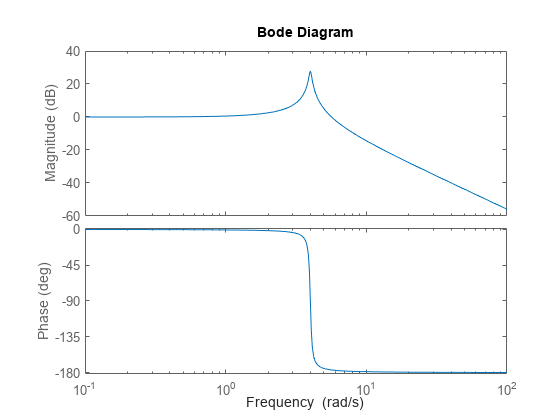
The plant model is a lightly damped, second-order system.

$$P(s)=\frac{16}{s^2+0.16s+16}$$.

A Bode plot shows the resonant peak.

P = tf(16,[1 0.16 16]);
bode(P)

Design Objectives and Initial Compensator Design

The design objectives for the closed-loop are the following.

In loop-shaping control design, you translate these requirements into a desired shape for the open-loop gain and seek a compensator that enforces this shape. For example, a compensator consisting of a PI term in series with a high-frequency lag component achieves the desired loop shape.

K_PI = pid(1,0.8);
K_rolloff = tf(1,[1/20 1]);
Kprop = K_PI*K_rolloff;
bodemag(P*Kprop); grid

Unfortunately, the compensator Kprop does not stabilize the closed-loop system. Examining the closed-loop dynamics shows poles in the right half-plane.

pole(feedback(P*Kprop,1))

ans = 4×1 complex

 -20.6975 + 0.0000i
   0.4702 + 5.5210i
   0.4702 - 5.5210i
  -0.4029 + 0.0000i

Enforcing Stability and Robustness with ncfsyn

You can use ncfsyn to enforce stability and adequate stability margins without significantly altering the loop shape. Use the initial design Kprop as loop-shaping pre-filter. ncfsyn assumes a positive feedback control system (see ncfsyn), so flip the sign of Kprop and of the returned controller.

[K,~,gamma] = ncfsyn(P,-Kprop);
K = -K;   % flip sign back
gamma

gamma = 
1.9903

A value of the performance gamma less than 3 indicates success (modest gain degradation along with acceptable robustness margins). The new compensator K stabilizes the plant and has good stability margins.

allmargin(P*K)

ans = struct with fields:
     GainMargin: [6.2984 10.9082]
    GMFrequency: [1.6108 15.0285]
    PhaseMargin: [79.9812 -99.6214 63.7590]
    PMFrequency: [0.4467 3.1469 5.2304]
    DelayMargin: [3.1253 1.4441 0.2128]
    DMFrequency: [0.4467 3.1469 5.2304]
         Stable: 1

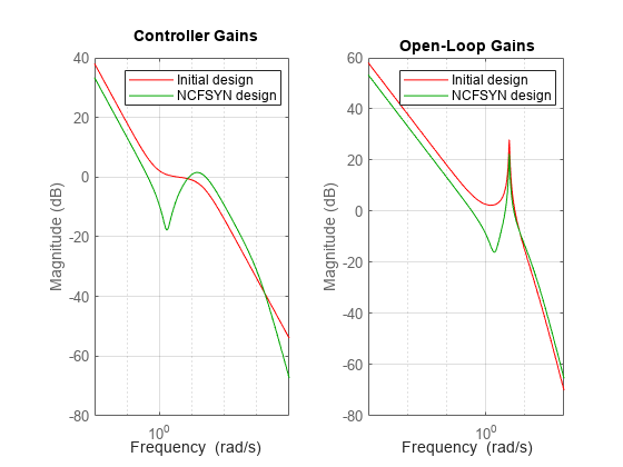
With gamma approximately 2, the expect at most 20*log10(gamma) = 6dB gain reduction in the high-gain region and at most 6dB gain increase in the low-gain region. The Bode magnitude plot confirms this. Note that ncfsyn modifies the loop shape mostly around the gain crossover to achieve stability and robustness.

subplot(1,2,1)
bodemag(Kprop,'r',K,'g',{1e-2,1e4}); grid
legend('Initial design','NCFSYN design')
title('Controller Gains')
subplot(1,2,2)
bodemag(P*Kprop,'r',P*K,'g',{1e-3,1e2}); grid
legend('Initial design','NCFSYN design')
title('Open-Loop Gains')

Figure 1: Compensator and open-loop gains.

Impulse Response

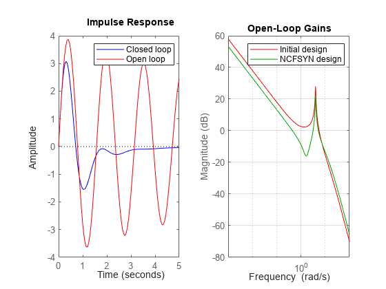
With the ncfsyn compensator, an impulse disturbance at the plant input is damped out in a few seconds. Compare this response to the uncompensated plant response.

subplot(1,2,1)
impulse(feedback(P,K),'b',P,'r',5);
legend('Closed loop','Open loop')

subplot(1,2,2);
impulse(-feedback(K*P,1),'b',5)
title('Control action')

Figure 2: Response to impulse at plant input.

Sensitivity Functions

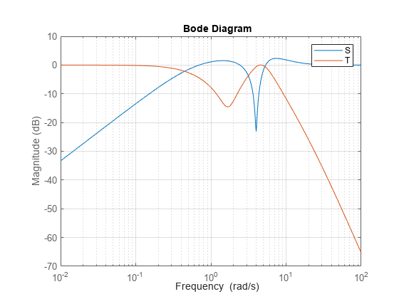
The closed-loop sensitivity and complementary sensitivity functions show the desired sensitivity reduction and high-frequency noise attenuation expressed in the closed-loop performance objectives.

S = feedback(1,P*K);
T = 1-S;
clf
bodemag(S,T,{1e-2,1e2}), grid
legend('S','T')

Conclusion

In this example, you used the function ncfsyn to adjust a hand-shaped compensator to achieve closed-loop stability while approximately preserving the desired loop shape.