Train DQN Agent with LSTM Network to Control House Heating System

This example shows how to train a deep Q-learning network (DQN) agent with a Long Short-Term Memory (LSTM) network to control a house heating system modeled in Simscape™. For more information on DQN agents, see Deep Q-Network (DQN) Agents.

House Heating Model

The reinforcement learning (RL) environment for this example uses a model from the House Heating System (Simscape) example. The model in this example contains a heater, a thermostat controlled by an RL agent, a house, outside temperatures, and a reward function. Heat is transferred between the outside environment and the interior of the home through the walls, windows, and roof. Weather station data between March 21 and April 15, 2022, from the MathWorks® campus in Natick, MA, is used to simulate the outside temperature. ThingSpeak™ was used to obtain this data. The data file temperatureMar21toApr15_20022.mat, is located in this example folder. For more information about the data acquisition, see Compare Temperature Data from Three Different Days (ThingSpeak).

The training goal for the agent is to minimize the energy cost and maximize the comfort of the room by turning on/off the heater. The house is comfortable when the room temperature ${\mathit{T}}_{\mathrm{room}}$is between ${\mathit{T}}_{\mathrm{comfortMin}}$ and ${\mathit{T}}_{\mathrm{comfortMax}}$.

The reinforcement learning problem is defined as follows:

• The observation is a 6-dimensional column vector that consists of the room temperature ($${}^{\circ }C$$) , outside temperature ($${}^{\circ }C$$) , maximum comfort temperature ($${}^{\circ }C$$) , minimum comfort temperature ($${}^{\circ }C$$) , last action, and price per kWh (USD). The maximum and minimum comfort temperatures and price per kWh in this example do not change over time, and you do not need to use them to train the agent. However, you can extend this example by varying these values over time.

• The action is discrete, and represents either turning the heater off (action is 0) or turning it on (action is 1).

• The total reward $\mathit{R}$ is calculated as the sum of the comfort reward $\mathit{Rc}$ and a penalty for switching $\mathit{Ps}$, to which an energy cost $\mathit{Ce}$ is subtracted: $\mathit{R}=\mathit{Rc}+\mathit{Ps}-\mathit{Ce}$. These three components are defines as follows.

$$\mathit{Rc}=\{\begin{array}{ll}0.1& \mathrm{if}{{\mathit{T}}_{\mathrm{comfortMin}}\le \mathit{T}}_{\mathrm{room}}\le {\mathit{T}}_{\mathrm{comfortMax}}\\ -\mathit{w}|{\mathit{T}}_{\mathrm{room}}-{\mathit{T}}_{\mathrm{comfortMin}}|& \mathrm{if}{\mathit{T}}_{\mathrm{room}}<{\mathit{T}}_{\mathrm{comfortMin}}\\ -\mathit{w}|{\mathit{T}}_{\mathrm{room}}-{\mathit{T}}_{\mathrm{comfortMax}}|& \mathrm{if}{\mathit{T}}_{\mathrm{room}}>{\mathit{T}}_{\mathrm{comfortMax}}\end{array}$$

where $\mathit{w}=0.1$, ${\mathit{T}}_{\mathrm{comfortMin}}=18,$ and ${\mathit{T}}_{\mathrm{comfortMax}}=23$.

$$\mathit{Ps}=\{\begin{array}{ll}-0.01& \mathrm{if}{\mathit{a}}_{\mathit{t}}\ne {\mathit{a}}_{\mathit{t}-1}\mathrm{where}{\mathit{a}}_{\mathit{t}}\mathrm{is}\mathrm{the}\mathrm{current}\mathrm{action}\mathrm{and}{\mathit{a}}_{\mathit{t}-1}\mathrm{is}\mathrm{the}\mathrm{previous}\mathrm{action}\\ 0& \mathrm{otherwise}\end{array}$$

$$\mathit{Ce}=\mathrm{CostPerStep}=\mathrm{PricePerKwh}*\mathrm{ElectricityUsed}$$

The reward function is inspired by [1].

• Is-Done signal is always 0, indicating that there is no early termination condition.

Open the model.

mdl = "rlHouseHeatingSystem";
open_system(mdl)

Define a sample time and the maximum number of steps per episode. Both variables are needed in the script and in the reset function.

sampleTime = 120; % seconds
maxStepsPerEpisode = 1000;

Assign the agent block path information to the agentBlk variable, for later use.

agentBlk = mdl + "/Smart Thermostat/RL Agent";

Load the outside temperature data to simulate the environment temperature.

data = load('temperatureMar21toApr15_2022.mat');
temperatureData = data.temperatureData;

Extract validation data.

temperatureMarch21 = temperatureData(1:60*24,:);
temperatureApril15 = temperatureData(end-60*24+1:end,:);

Extract training data.

 temperatureData = temperatureData(60*24+1:end-60*24,:);

The Simulink® model loads the following variables as a part of observations.

outsideTemperature = temperatureData;
comfortMax = 23;
comfortMin = 18;

Define observation and action specifications.

obsInfo = rlNumericSpec([6,1]);
actInfo = rlFiniteSetSpec([0,1]); % (0=off,1=on)

The actor and critic networks of the DQN agent are initialized randomly. Ensure reproducibility by fixing the seed of the random generator.

rng(0)

Create DQN Agent with LSTM Network

DQN agents use a parametrized Q-value function approximator to estimate the value of the policy. Since DQN agents have a discrete action space, you have the option to create a vector (that is multi-output) Q-value function critic, which is generally more efficient than a comparable single-output critic.

A vector Q-value function takes only the observation as input and returns as output a single vector with as many elements as the number of possible actions. The value of each output element represents the expected discounted cumulative long-term reward when an agent starts from the state corresponding to the given observation and executes the action corresponding to the element number (and follows a given policy afterwards).

Specify training options for the critic and the actor using rlOptimizerOptions.

criticOpts = rlOptimizerOptions( ...
    LearnRate=0.001, ...
    GradientThreshold=1);

Specify the DQN agent options using rlDQNAgentOptions, include the training options for the critic.

agentOpts = rlDQNAgentOptions(...
    UseDoubleDQN = false, ...    
    TargetSmoothFactor = 1, ...
    TargetUpdateFrequency = 4, ...   
    ExperienceBufferLength = 1e6, ...
    CriticOptimizerOptions = criticOpts, ...
    MiniBatchSize = 64);

You can also set or modify the agent options using dot notation.

agentOpts.EpsilonGreedyExploration.EpsilonDecay = 0.0001;

To model the parametrized Q-value function within the critic, use a recurrent neural network, which can capture the effect of previous observations. By setting the UseRNN option in rlAgentInitializationOptions, you can create a default DQN agent with an LSTM network. Alternatively, you can manually configure the LSTM network. See Water Distribution System Scheduling Using Reinforcement Learning to create an LSTM network for the DQN agent manually.

useRNN = true;
initOpts = rlAgentInitializationOptions( ...
    UseRNN=useRNN, ...
    NumHiddenUnit=64);

When using a recurrent neural network, you must set SequenceLength to be greater than 1 in rlDQNAgentOptions. This option is used in training to determine the length of the minibatch used to calculate the gradient. For more information about LSTM layers, see Long Short-Term Memory Neural Networks.

if useRNN
    agentOpts.SequenceLength = 20;
end

Create a DQN agent with default critic network using rlDQNAgent, the agent initialization options object (which specify that a recurrent network is needed), and the agent options object.

agent = rlDQNAgent(obsInfo, actInfo, initOpts, agentOpts);

You can also modify the agent options, including the critic options, using dot notation. For example, specify the agent sample time.

agent.SampleTime = sampleTime;

Define Simulink Environment

Create an environment interface for the house heating environment.

env = rlSimulinkEnv(mdl,agentBlk,obsInfo,actInfo);

Use hRLHeatingSystemResetFcn to reset the environment at the beginning of each episode. This function randomly selects the time between March 22nd and April 14th. The environment uses this time as the initial time for the outside temperatures.

env.ResetFcn = @(in) hRLHeatingSystemResetFcn(in);

Validate the environment.

validateEnvironment(env)

Train Agent

To train the agent, first specify the training options. For this example, use the following options.

• Run training for at most 150 episodes, with each episode lasting 1000 time steps.

• Set the Plots option to "training-progress", which displays training progress in the Reinforcement Learning Training Monitor

• Set the Verbose option to false to disable the command line display.

• Stop training when the agent receives an average cumulative reward greater than 85 over 5 consecutive episodes.

For more information, see rlTrainingOptions.

trainOpts = rlTrainingOptions(...
    MaxEpisodes = 150, ...
    MaxStepsPerEpisode = maxStepsPerEpisode, ...
    ScoreAveragingWindowLength = 5,...    
    Verbose = false, ...
    Plots = "training-progress",...
    StopTrainingCriteria = "AverageReward",...
    StopTrainingValue = 85);

Train the agent using the train function. Training this agent is a computationally-intensive process that takes several hours to complete. To save time while running this example, load a pretrained agent by setting doTraining to false. To train the agent yourself, set doTraining to true.

doTraining = false;
if doTraining
    % Train the agent.
    trainingStats = train(agent,env,trainOpts);
else
    % Load the pretrained agent for the example.
    load("HeatControlDQNAgent.mat","agent")
end

Simulate DQN Agent

To validate the performance of the trained agent, simulate it within the house heating system. For more information on agent simulation, see rlSimulationOptions and sim.

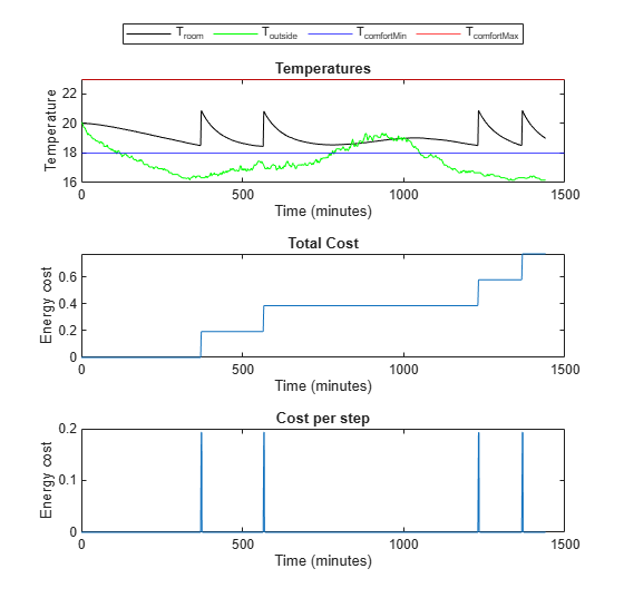
First, evaluate the agent's performance using the temperature data from March 21st, 2022. The agent did not use this temperature data for training.

maxSteps= 720;
validationTemperature = temperatureMarch21;
env.ResetFcn = @(in) hRLHeatingSystemValidateResetFcn(in);
simOptions = rlSimulationOptions(MaxSteps = maxSteps);
experience1 = sim(env,agent,simOptions);

Use the localPlotResults function, provided at the end of the example, to analyze the performance.

localPlotResults(experience1, maxSteps, ...
    comfortMax, comfortMin, sampleTime,1)

Comfort Temperature violation: 0/1440 minutes, cost: 7.707458 dollars

Next, evaluate the agent's performance using the temperature data from April 15th, 2022. The agent did not use this temperature data during training either.

% Validate agent using the data from April 15
validationTemperature = temperatureApril15;
experience2 = sim(env,agent,simOptions);
localPlotResults( ...
    experience2, ...
    maxSteps, ...
    comfortMax, ...
    comfortMin, ...
    sampleTime,2)

Comfort Temperature violation: 0/1440 minutes, cost: 7.925062 dollars

Evaluate the agent's performance when the temperature is mild. Add eight degrees to the temperature from April 15th to create data for mild temperatures.

% Validate agent using the data from April 15 + 8 degrees
validationTemperature = temperatureApril15;
validationTemperature(:,2) = validationTemperature(:,2) + 8;
experience3 = sim(env,agent,simOptions);
localPlotResults(experience3, ...
    maxSteps, ...
    comfortMax, ...
    comfortMin, ...
    sampleTime, ...
    3)

Comfort Temperature violation: 0/1440 minutes, cost: 0.195658 dollars

Local Function

function localPlotResults(experience, maxSteps, comfortMax, comfortMin, sampleTime, figNum)
    % localPlotResults plots results of validation

    % Compute comfort temperature violation
    minutesViolateComfort = ...
    sum(experience.Observation.obs1.Data(1,:,1:maxSteps) < comfortMin) ...
    + sum(experience.Observation.obs1.Data(1,:,1:maxSteps) > comfortMax);
    
    % Cost of energy
    totalCosts = experience.SimulationInfo(1).househeat_output{1}.Values;
    totalCosts.Time = totalCosts.Time/60;
    totalCosts.TimeInfo.Units="minutes";
    totalCosts.Name = "Total Energy Cost";
    finalCost = experience.SimulationInfo(1).househeat_output{1}.Values.Data(end);

    % Cost of energy per step
    costPerStep = experience.SimulationInfo(1).househeat_output{2}.Values;
    costPerStep.Time = costPerStep.Time/60;
    costPerStep.TimeInfo.Units="minutes";    
    costPerStep.Name = "Energy Cost per Step";
    minutes = (0:maxSteps)*sampleTime/60;

    % Plot results   

    fig = figure(figNum);
    % Change the size of the figure
    fig.Position = fig.Position + [0, 0, 0, 200];

    % Temperatures
    layoutResult = tiledlayout(3,1);
    nexttile
    plot(minutes, ...
        reshape(experience.Observation.obs1.Data(1,:,:), ...
        [1,length(experience.Observation.obs1.Data)]),"k")
    hold on
    plot(minutes, ...
        reshape(experience.Observation.obs1.Data(2,:,:), ...
        [1,length(experience.Observation.obs1.Data)]),"g")
    yline(comfortMin,'b')
    yline(comfortMax,'r')
    lgd = legend("T_{room}", "T_{outside}","T_{comfortMin}", ...
        "T_{comfortMax}","location","northoutside");
    lgd.NumColumns = 4;
    title("Temperatures")
    ylabel("Temperature")
    xlabel("Time (minutes)")
    hold off

    % Total cost
    nexttile
    plot(totalCosts)    
    title("Total Cost")
    ylabel("Energy cost")

    % Cost per step
    nexttile
    plot(costPerStep)  
    title("Cost per step")
    ylabel("Energy cost")    
    fprintf("Comfort Temperature violation:" + ...
        " %d/1440 minutes, cost: %f dollars\n", ...
        minutesViolateComfort, finalCost);
end

Reference

[1] Du, Yan, Fangxing Li, Kuldeep Kurte, Jeffrey Munk, and Helia Zandi. “Demonstration of Intelligent HVAC Load Management With Deep Reinforcement Learning: Real-World Experience of Machine Learning in Demand Control.” IEEE Power and Energy Magazine 20, no. 3 (May 2022): 42–53. https://doi.org/10.1109/MPE.2022.3150825.