Scattering Problem

Solve a simple scattering problem, where you compute the waves reflected by an object illuminated by incident waves. This example shows how to solve a scattering problem using the electromagnetic workflow. For the general PDE workflow, see Helmholtz Equation on Disk with Square Hole.

For this problem, assume that the domain is an infinite horizontal membrane that is subjected to small vertical displacements. The membrane is fixed at the object boundary. The medium is homogeneous, and the phase velocity (propagation speed) of a wave, $\alpha$, is constant. For this problem, assume $\alpha$=1. In this case, the frequency wave number equals the frequency, $\mathit{k}=\omega /\alpha =\omega$.

Specify the frequency as $4\pi$.

omega = 4*pi;

Represent the square surface with a diamond-shaped hole. Define a diamond in a square, place them in one matrix, and create a set formula that subtracts the diamond from the square.

square = [3; 4; -5; -5; 5; 5; -5; 5; 5; -5];
diamond = [2; 4; 2.1; 2.4; 2.7; 2.4; 1.5; 1.8; 1.5; 1.2];
gd = [square,diamond];
ns = char('square','diamond')';
sf = 'square - diamond';

Create the geometry.

g = decsg(gd,sf,ns);

Plot the geometry with the edge labels.

figure; 
pdegplot(g,EdgeLabels="on"); 
xlim([-6,6])
ylim([-6,6])

Create an femodel object for harmonic analysis with the electric field type. Include the geometry into the model.

model = femodel(AnalysisType="electricHarmonic", ...
                Geometry=g);

Specify the vacuum permittivity and permeability values as 1.

model.VacuumPermittivity = 1;
model.VacuumPermeability = 1;

Specify the relative permittivity, relative permeability, and conductivity of the material.

model.MaterialProperties = ...
    materialProperties(RelativePermittivity=1, ...
                       RelativePermeability=1, ...
                       ElectricalConductivity=0);

Apply the absorbing boundary condition on the edges of the square. Specify the thickness and attenuation rate for the absorbing region by using the Thickness, Exponent, and Scaling arguments.

ffbc = farFieldBC(Thickness=2,Exponent=4,Scaling=1);
model.EdgeBC(1:4) = edgeBC(FarField=ffbc);

Apply the boundary condition on the diamond edges.

innerBCFunc = @(location,~) [-exp(-1i*omega*location.x); ...
                            zeros(1,length(location.x))];
model.EdgeBC(5:8) = edgeBC(ElectricField=innerBCFunc);

Generate a mesh.

model = generateMesh(model,Hmax=0.1);

Solve the harmonic analysis model for the frequency $\omega =4\pi$.

result = solve(model,omega);

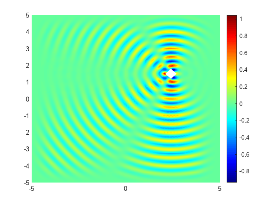
Plot the real part of the x-component of the resulting electric field.

u = result.ElectricField;

figure
pdeplot(result.Mesh, ...
        XYData=real(u.Ex), ...
        Mesh="off");
colormap(jet)

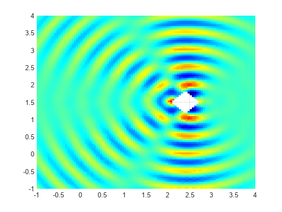
Interpolate the resulting electric field to a grid covering the portion of the geometry, for x and y from -1 to 4.

v = linspace(-1,4,101);
[X,Y] = meshgrid(v);
Eintrp = interpolateHarmonicField(result,X,Y);

Reshape Eintrp.Ex and plot the x-component of the resulting electric field.

EintrpX = reshape(Eintrp.ElectricField.Ex,size(X));

figure
surf(X,Y,real(EintrpX),LineStyle="none");
view(0,90)
colormap(jet)

Using the solutions for a vector of frequencies, create an animation showing the corresponding solution to the time-dependent wave equation.

result = solve(model,omega/10:omega);
figure
for m = 1:length(omega/10:omega)
    u = result.ElectricField;
    msh = result.Mesh;
    pdeplot(msh,XYData=real(u.Ex(:,m)),Mesh="off");
    colormap(jet)
    M(m) = getframe;
end

To play the animation, use the movie function. For example, to play the animation five times in a loop with 3 frames per second, use the movie(M,5,3) command.